Legal Probabilism with Bayesian Networks and R
Brief description
The entry on Legal Probabilism in the Stanford Encyclopedia of Philosophy which I co-authored with Marcello Di Bello includes a section on Bayesian networks. Here, I provide more details and source code in R for the examples discussed in that section.
This work was funded by the National Science Center (grant no. 2021/41/B/HS1/01814).
-
If you just want to get the code, here is the folder with $\textsf{R}$ files containing bare code for the BNs and the wrapper functions.
-
If you prefer to look at the code with some explanation of what’s going on and why, read on, feel free to skip the last section.
-
If you’re interested in a few words of a more theoretical explanation, read the last section with mathy details first.
Recommended readings
Before we move on, if you’re interested in BNs, here are three really good sources to get you started:
-
“Bayesian Networks and Probabilistic Inference in Forensic Science” by Taroni, Aitken, Garbolino and Biedermann. This is clearly the one with forensic science in the focus.
-
For the more mathematically minded, “Learning Bayesian Networks” by Neapolitan is pretty awesome.
-
For a very accessible and fascinating account of the multiplicity of applications of Bayesian Neworks, check our “Risk Assessment and Decision Analysis with Bayesian Networks” by Fenton and Neil.
-
They don’t contain R code, though. For a great treatment on the use of
bnlearnpackage, read “Bayesian Networks With Examples in R” by Marco Scutari and Jean-Baptiste Denis.
Contents
- Brief description
- Recommended readings
- Set-up
- Qualitative BNs (DAGs with node labels)
- Adding conditional probability tables (CPTs) to obtain BNs
- Legal idioms
- BNs for mixed DNA evidence evaluation
- A BN for the Sally Clark case
- Scenarios with BNs
- Mathy details
The examples are given in R code, which we intertwine with additional explanations, which the reader is welcome to skip if they look familiar.
Set-up
First, you need to install the relevant R libraries. The crucial one is bnlearn by Marco Scutari (who was also kind enough to include some functionalities when I inquired about them). This is a bit
tricky, because some of them have to be installed through BiocManager.
One way to go is this:
install.packages("https://www.bnlearn.com/releases/bnlearn_latest.tar.gz", repos = NULL, type = "source")
install.packages("BiocManager")
if (!requireNamespace("BiocManager", quietly = TRUE))
  install.packages("BiocManager")
BiocManager::install()
BiocManager::install(c("graph", "Rgraphviz"))

install.packages("https://www.bnlearn.com/releases/bnlearn_latest.tar.gz", repos = NULL, type = "source")
Then load the libraries we use (you need to have them installed first):
library(bnlearn)
library(Rgraphviz)
Qualitative BNs (DAGs with node labels)
Instead, we start with representing dependencies between random variables in such a set by means of a directed acyclic graph (DAG). A DAG is a collection of nodes (called also vertices) – think of them as corresponding to the RVs, directed edges (also called arcs; they can be thought of as ordered pairs of nodes), such that there is no sequence of nodes $v_0,\dots, v_k$ with edges from $v_i$ to $v_{i+1}$ for $0\leq i\leq k-1$ with $v_0=v_k$. (Sometimes it is also required that the graph should be connected: that for any two nodes there is an undirected path between them.) A qualitative BN (QBN) is a DAG with nodes labeled by RVs.
Here’s one example of a QBN:
cancer1 <- empty.graph(nodes = c("PS","SH","S","C"))
cancer1.arcs <- matrix(c("PS", "SH",
                   "PS", "S",
                   "SH", "C",
                    "S", "C"),
                 byrow = TRUE, ncol = 2,
                 dimnames = list(NULL, c("from", "to")))
arcs(cancer1) = cancer1.arcs
graphviz.plot(cancer1)
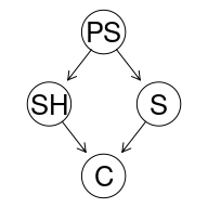
With the intended reading:
| RV | Proposition |
|---|---|
| PS | At least one parent smokes. |
| SH | The subject is a second-hand smoker. |
| S | The subject smokes. |
| C | The subject develops cancer. |
This can be achieved in a somewhat simpler manner like this:
cancer2DAG <- model2network("[SH|PS][PS][S|PS][C|SH:S]")
graphviz.plot(cancer2DAG)
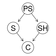
The ancestors of $C$ are all the other RVs, the parents of $C$ are $SH$ and $S$, the descentants of $PS$ are all the other RVs, and the children of $PS$ are $SH$ and $S$.
The edges, intuitively, are meant to capture direct influence between RVs. The role that such direct influence plays is that in a BN any RV is conditionally independent of its nondescentants (including ancestors), given its parents. If this is the case for a given probabilistic measure $P{}$ and a given DAG $\mathsf{G}$, we say that $P{}$ is compatible with $\mathsf{G}$, or that it satisfies the Markov condition.
Adding conditional probability tables (CPTs) to obtain BNs
A quantitative BN (further on, simply BN) is a DAG with CPTs, and we say that it represents a probabilistic measure $\mathsf{P}$ quantitatively just in case they are compatible, and $\mathsf{P}$ agrees with its assignment of CPTs.
Adding probabilities to the DAG we already have can be achieved easily using a bunch of wrappers we wrote for root nodes, and single- and double-parented nodes. First, load the script (in needs to be in your folder), then, remember that E stands for the child, and H for a parent. We assume states are binary, and so S1 corresponds to a state occuring and S2 to it failing to occur. So, for instance, if we have h1Node = "S", h2Node = "SH" then probEifH1S1H2S1 = .6 means the probability of the child note (E) if the first hypothesis (S) is true (S1) and the second hypothesis (SH) is true as well (S1).
source("cptCreate.R")

#tables for separate nodes
PSprob <- priorCPT("PS",prob1 = .3)

Sprob <-  singleCPT(eNode = "S", hNode = "PS", probEifHS1 = .4 , probEifHS2 =  .2)
SHprob <- singleCPT(eNode = "SH", hNode = "PS", probEifHS1 = .8, probEifHS2 = .3)

Cprob <- doubleCPT(eNode= "C", h1Node = "S", h2Node = "SH",
                   probEifH1S1H2S1 = .6,
                   probEifH1S1H2S2 = .4,
                   probEifH1S2H2S1 = .1,
                   probEifH1S2H2S2 = .01)

#put them together and add to the DAG to create a BN
cancerCPT <- list(PS = PSprob, S = Sprob, SH = SHprob, C = Cprob)
cancerBN <- custom.fit(cancer2DAG,cancerCPT)

#display the CPTs for all the nodes
cancerBN
##
##   Bayesian network parameters
##
##   Parameters of node C (multinomial distribution)
##
## Conditional probability table:
##
## , , SH = 1
##
##    S
## C      1    0
##   1 0.60 0.10
##   0 0.40 0.90
##
## , , SH = 0
##
##    S
## C      1    0
##   1 0.40 0.01
##   0 0.60 0.99
##
##
##   Parameters of node PS (multinomial distribution)
##
## Conditional probability table:
##  PS
##   1   0
## 0.3 0.7
##
##   Parameters of node S (multinomial distribution)
##
## Conditional probability table:
##
##    PS
## S     1   0
##   1 0.4 0.2
##   0 0.6 0.8
##
##   Parameters of node SH (multinomial distribution)
##
## Conditional probability table:
##
##    PS
## SH    1   0
##   1 0.8 0.3
##   0 0.2 0.7
How do you read this?
-
Let’s look at the parameters of node
PSfirst. The table tells you that the prior probability of at least one parent smoking is .3. -
For
SandSHthe table is 2-dimensional; the tables tell you the probabilies of various states of these nodes conditional on the state of the single parent node. For instance, the probability that the patient smokes given that at least one of their parents smokes is .4, while the probability that a patient is a second-hand smoker given that their parents smoke is .8 (and .3 otherwise). -
The table for
Cis three-dimensional, so $\mathsf{R}$ splits it onto layers. In one, we assume the subject is a second-hand smoker (SH=1), and in the second layer that they are not (SH=0). In each layer, the conditonal probability ofCgiven two possible states ofSis given.
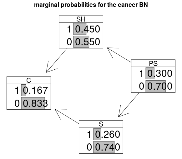
The BN can be plotted with the resulting marginal probabilties as follows:
graphviz.chart(cancerBN, grid = FALSE, type = "barprob", layout = "neato", scale = c(1,1.5),
               main="marginal probabilities for the cancer BN")
Legal idioms
The idea that BNs can be used for probabilistic reasoning in legal fact-finding started gaining traction in late eighties (Edwards 1991). It gained some (albeit limited) traction with the work of many researchers, including the works of Neil, Fenton, and Nielsen and Hepler, Dawid and Leucari, reaching a fairly advanced stage with the monograph by Taroni, Aitken, Garbonino & Biedermann.
Hypothesis-evidence
One reccuring pattern captures the relation between a hypothesis and a piece of evidence, the idea being that it is whether the hypothesis is true that caused the (non-)occurence of the evidence.
HE <- model2network("[Evidence|Hypothesis][Hypothesis]")
graphviz.plot(HE)
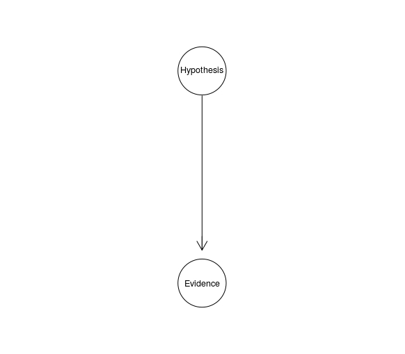
For instance, $H$ might take values from the range of $1-40$, the distance in meters from which the gun has been shot, and $E$ might be a continuous variable representing the density of gun shot residues. (This example also indicates that RVs don’t have to be binary for legal applications.)
Another example, this time with binary variables, takes $H$ to be the claim that the supect is guilty and $E$ the presence of a DNA match with a crime scene stain. One way the CPTs could look like in this case is this:
Hypothesis.prob <-  array(c(0.01, 0.99), dim = 2, dimnames = list(HP =  c("guilty","not guilty")))

Evidence.prob <- array(c( 0.99999, 0.00001, 0, 1), dim = c(2,2),dimnames = list(Evidence = c("DNA match","no match"),
      Hypothesis = c("guilty","not guilty")))

HEcpt <- list(Hypothesis=Hypothesis.prob,Evidence=Evidence.prob)
HEbn = custom.fit(HE,HEcpt)
| guilty | not guilty | |
|---|---|---|
| DNA match | 0.99999 | 0 |
| No match | 0.00001 | 1 |
Two pieces of evidence
The true power of BNs, however, appears when we go beyond a simple two-node situations for which calculations can be done by hand. For instance, imagine we have two pieces of evidence: a DNA match, and a witness testimony. The DAG might look like this:
HEE.dag <- model2network("[H][W|H][DNA|H]")
graphviz.plot(HEE.dag)
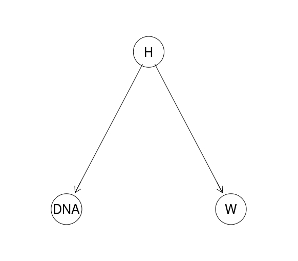
The CPTs can, for instance, be as follows:
HEEdag <- model2network("[H][W|H][DNA|H]")
Hprob <- array(c(0.01, 0.99), dim = 2,
                dimnames = list(h = c("murder","nomurder")))

Wprob <- array(c( 0.7, 0.3, 0.4, 0.6), dim = c(2,2),dimnames =
              list(W= c("seen","notseen"), H = c("murder","nomurder")))

DNAprob <- array(c( 1, 0, 0.001, 0.999), dim = c(2,2),
                  dimnames = list(DNA =c("dnamatch","nomatch"),
                                  H = c("murder","nomurder")))

HEEcpt <- list(H=Hprob,W=Wprob,DNA = DNAprob)

HEEbn <- custom.fit(HEEdag,HEEcpt)
| Pr(H) | |
|---|---|
| murder | 0.01 |
| no.murder | 0.99 |
| H=murder | H=no.murder | |
|---|---|---|
| W=seen | 0.7 | 0.4 |
| W=not.seen | 0.3 | 0.6 |
| H=murder | H=no.murder | |
|---|---|---|
| DNA=match | 1 | 0.001 |
| DNA=no.match | 0 | 0.999 |
The CPT for the hypothesis contains the prior probability that a murder has been commited by the suspect. The CPTs for the other variables include (made up) probabilities of a DNA match and of a witness seeing the suspect near the crime scene at an appropriate time conditional on various states of the murder hypothesis: $\mathsf{P} (\textrm{W=seen}\vert \textrm{H=murder})=0.7, \mathsf{P} (\textrm{W=seen}\vert \textrm{H=no.murder})=0.4$ etc.
Calculating posteriors and visualising updated BNs
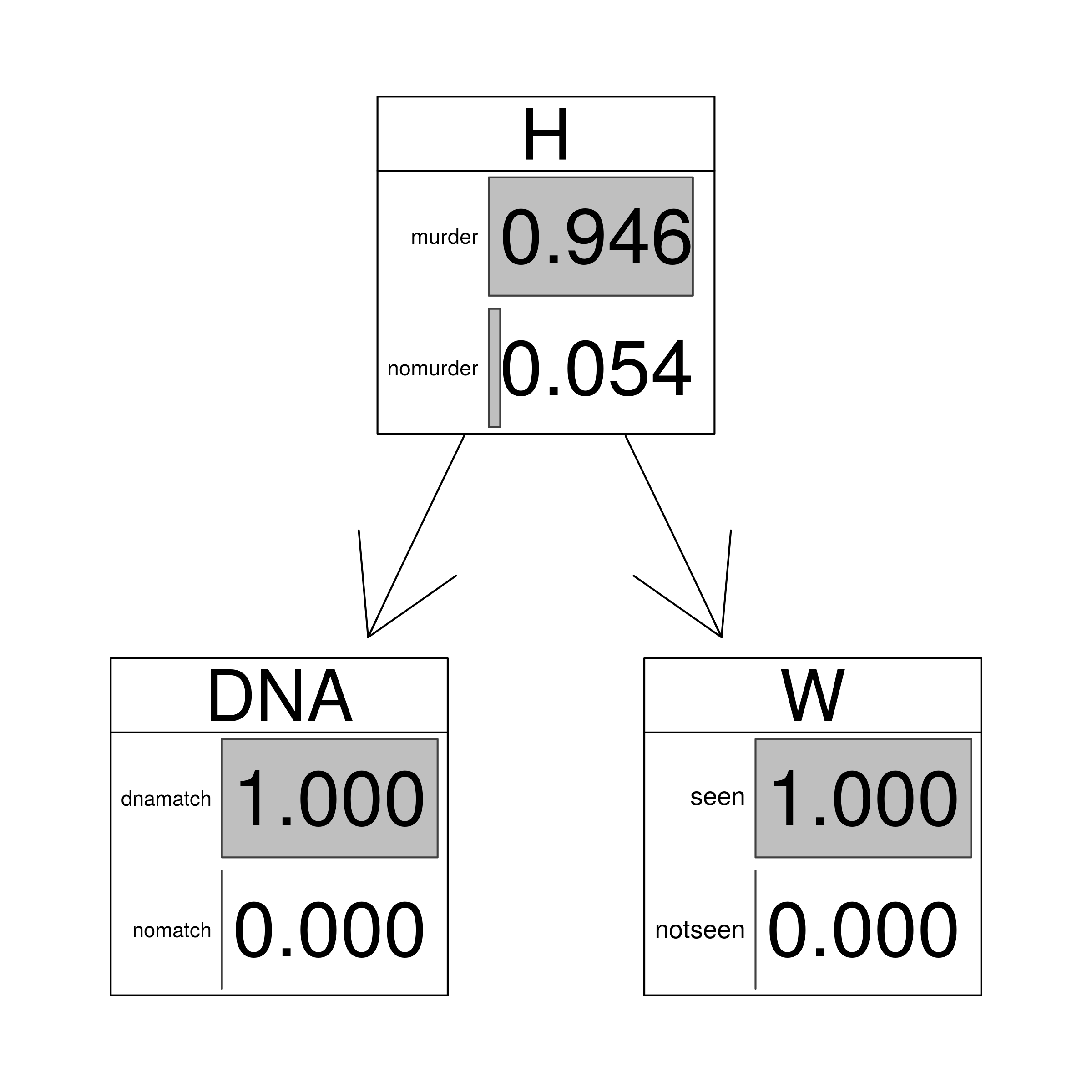
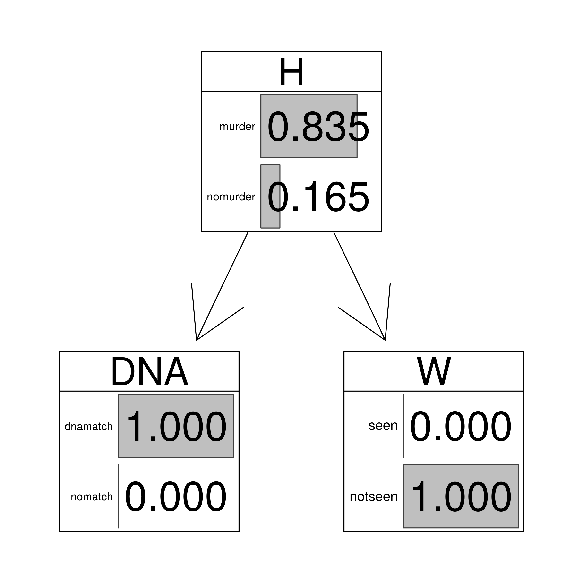
This BN is fairly simple, yet correct intuitive assessment of how the probability of the hypothesis depends on various states of the evidence is already rather difficult. Moreover, already at this level of complexity formula-based calculations by hand also become cumbersome. In contrast, a fairly straightforward use of a dedicated piece of software to the BN will easily lead to the following results:
| DNA | W | $\mathsf{P} (H)$ |
|---|---|---|
| match | seen | 0.9464 |
| match | not.seen | 0.8347 |
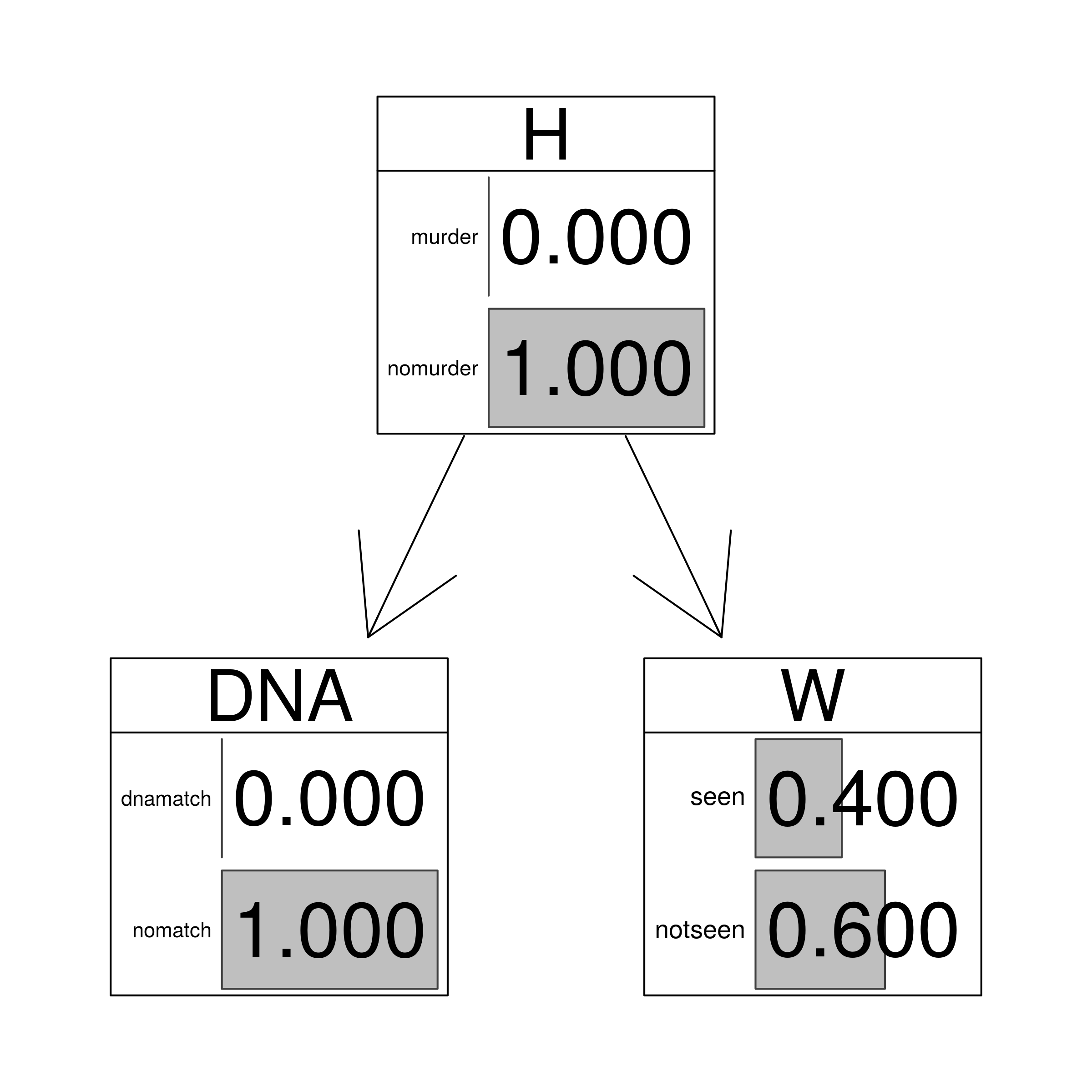
| no.match | either | 0 |
But how did we get these values? Well, we first convert the BNs to junction trees for calculations, then update them with evidence, and query about the values.
library(bnlearn)
library(gRain)
junction <- compile(as.grain(HEEbn))

junctionMS <- setEvidence(junction, nodes = c("DNA","W"), states = c("dnamatch","seen") )
querygrain(junctionMS)$H
## H
##     murder   nomurder
## 0.94645754 0.05354246
junctionMN <- setEvidence(junction, nodes = c("DNA","W"), states = c("dnamatch","notseen"))
querygrain(junctionMN)$H
## H
##    murder  nomurder
## 0.8347245 0.1652755
junctionNOMATCH <- setEvidence(junction, nodes = c("DNA"), states = c("nomatch"))
querygrain(junctionNOMATCH)$H
## H
##   murder nomurder
##        0        1
Moreover, we can convert the updated junction trees back to bayesian networks and use them for visualisation:
HEEms <- as.bn.fit(junctionMS, including.evidence = TRUE)
HEEmn <- as.bn.fit(junctionMN, including.evidence = TRUE)
HEEnomatch <- as.bn.fit(junctionNOMATCH, including.evidence = TRUE)

graphviz.chart(HEEms, grid = FALSE, type = "barprob",  scale = c(2,2),
               main=" DNA match and  witness evidence")

graphviz.chart(HEEmn, grid = FALSE, type = "barprob",  scale = c(2,2),
               main="DNA match and  negative witness evidence")

graphviz.chart(HEEnomatch, grid = FALSE, type = "barprob",  scale = c(2,2),
               main="Exclusionary DNA match and  no witness evidence")
Cause, measurement, synthesis
The Cause-Consequence Idiom models a causal process in terms of the relationship between a cause and its consequence.
CauseCon <-  model2network("[Cause][Consequence|Cause]")
graphviz.plot(CauseCon)
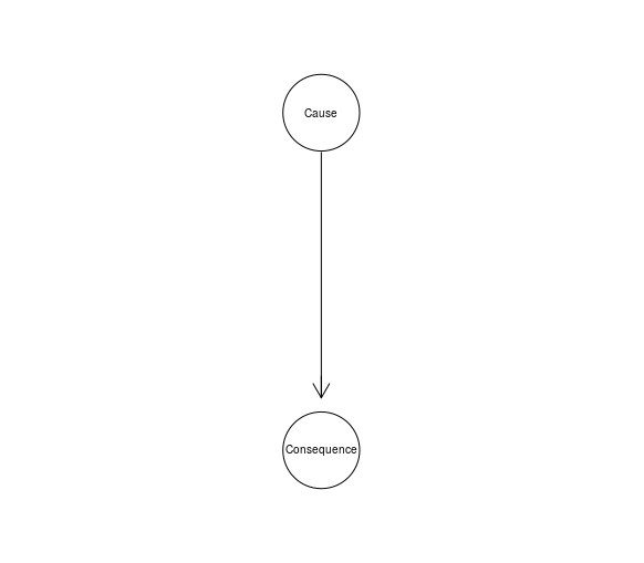
In fact, a BN fragment for a hypothesis-evidence relationship often instantiates this idiom, because often there is a causal relationship between the hypothesis and the evidence.
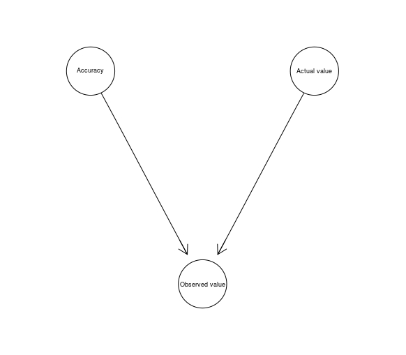
The Measurement Idiom is used to represent the uncertainty arising from the way a given variable is measured.
Measurement <- model2network("[Accuracy][Actual value][Observed value|Accuracy:Actual value]")
graphviz.plot(Measurement)
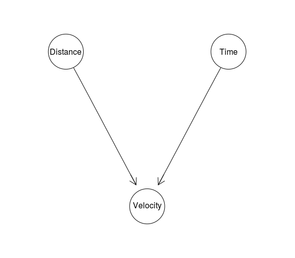
Definitional/Synthesis Idiom is used in situations in which a node is defined in terms of its parents nodes. For instance:
Definitional <- model2network("[Distance][Time][Velocity|Distance:Time]")
graphviz.plot(Definitional)
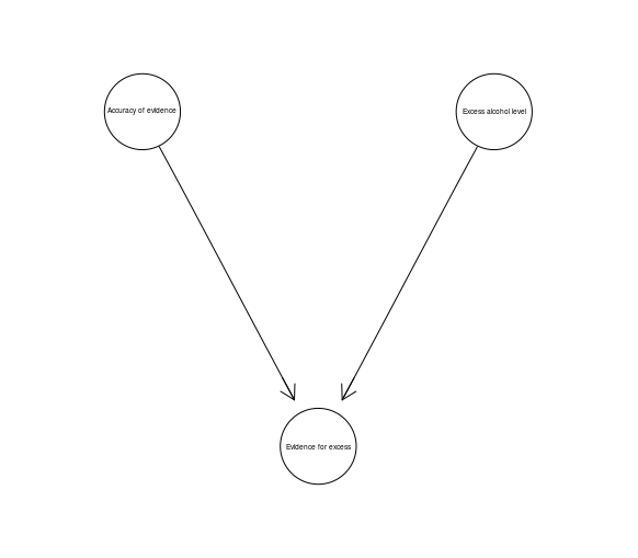
We already discussed one idiom: The Evidence Idiom, which simply consists of a hypothesis node, and various pieces of evidence related to it as its children. The legal variant of the Measurement Idiom is called the Evidence Accuracy Idiom, and its instantiation might look like this:
Evidence accuracy, opportunity
We already discussed the evidence idiom, which simply consists of a hypothesis node, and various pieces of evidence related to it as its children. The legal variant of the Measurement Idiom is called the Evidence Accuracy Idiom, and its instantiation might look like this:
evidenceAccuracy <-  model2network("[Accuracy of evidence][Excess alcohol level][Evidence for excess|Accuracy of evidence:Excess alcohol level]")
graphviz.plot(evidenceAccuracy)
A novelty appears, however, when we think about the notion of opportunity understood as a necessary requirement for the defendat’s guilt (such as being present at the scene). Oppotrunity is built in as a parent of the guilt hypothesis, here’s an example with a few moving elements:
opportunity <- model2network("[H1][H2|H1][A1][A2][E1|H1:A1][E2|H1:A2]")
graphviz.plot(opportunity)
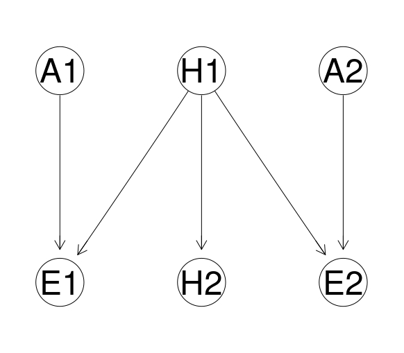
| Node | Proposition |
|---|---|
| H1 | Defendant present at the scene |
| H2 | Defendant guilty |
| A1 | Accuracy of eyewitness evidence |
| A2 | Accuracy of security camera evidence |
| E1 | Eyewitness testimony |
| E2 | Evidence from security camera |
The same structure is used to build in a node for a motive.
Dependency between items of evidence, alibi
One useful aspect of BN representation is that we can clearly visualise and take under consideration the dependency between pieces of evidence. For instance, if one of two security cameras captured an image of someone matching the suspect, it might be very likely that so did the second one. In such cases, additional evidence might be practically useless and presenting it as independent might lead to gross overestimation of its importance.
cameras <- model2network("[H][D][C1|H][C2|H:C1:D]")
graphviz.plot(cameras)
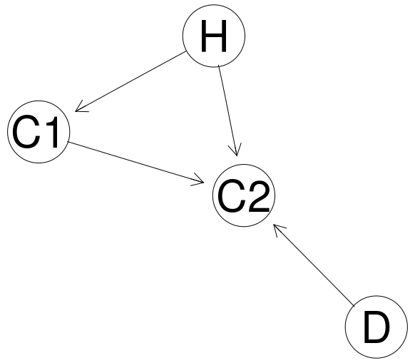
| Node | Proposition |
|---|---|
| H | Defendant present at the scene |
| C1 | Camera 1 captures image of a matching person |
| C2 | Camera 2 captures image of a matching person |
| D | What cameras capture is dependent |
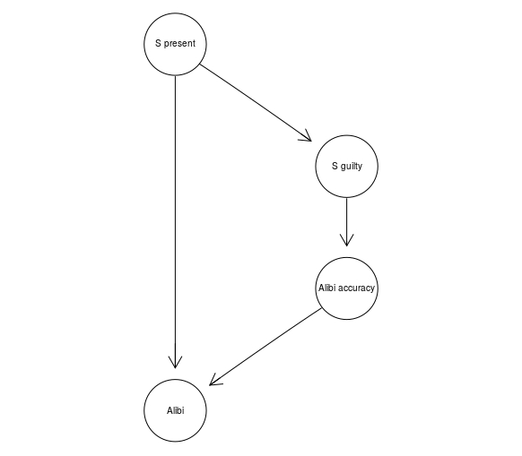
The Alibi Idiom, on the other hand, is used to model alibi evidence which seems to directly contradict the prosecution hypothesis. Crucially, the hypothesis itself may have impact on the accuracy of the evidence:
alibi <- model2network("[S present][S guilty|S present][Alibi accuracy|S guilty][Alibi|Alibi accuracy:S present]")
graphviz.plot(alibi)
BNs for mixed DNA evidence evaluation
One type of legal applications of BNs is to evaluate DNA evidence. At each locus (a small region of the DNA) there occur short sequences of base pairs repeated multiple times. The number of times that the sequences are repeated varies between individuals. The length of a repeated sequences expressed as the number of repeats in the sequence is called an allele. At each locus there are two alleles, iherited from the parents. So a particular locus can be described in terms of two numbers, the genotype of that locus. The pairs can be the same (the person is then homozygous at that locus) or diferent (the person is then heterozygous). Normally, a genotype at a given locus is shared by 5-15% of the population. A DNA profiling system consists of a selection of loci (often 17 or 20). Information about genotypes at those loci together with their frequencies is then used to estimate the frequency of a given DNA profile. On the rather uncontroversial assumption of the independence of the loci used in DNA profiling, this is usually done by multiplying probabilities for each particular genotype.
However, in practice, there are complications. If people are related, they are more likely to share genotypes. Moreover, sometimes a sample from the crime scene is of low quality and only a subset of the usual loci can be used. Finally, a profile can be mixed and involve DNA sample containing material from more than one individual. For instance, if three different alleles are found at locu TH01 (say, 7,8,9), it is clear that the profile is mixed. Say now the suspect S has genotype (7,7). The complication now is that there are many possible combinations of the DNA (and only one of them doesn’t exclude the suspect):
| Contributor 1 (C1) | Contributor 2 (C2) |
|---|---|
| (7,7) | (8,9) |
| (7,8) | (8,9) |
| (7,8) | (9,9) |
| (7,8) | (9,9) |
| (8,8) | (7,9) |
To properly evaluate this piece of evidence, the following BN can be used:
DNA789 <- model2network("[S is C1][S is C2][Genotype of C1|S is C1][Genotype of C2|S is C2][S is the source|S is C1:S is C2][(7,8,9) found|Genotype of C1:Genotype of C2]")
graphviz.plot(DNA789)
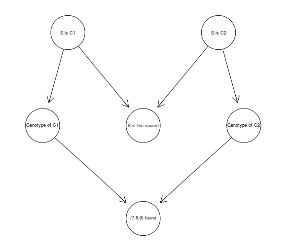
to establish that such evidence causes only a small increase of the source hypothesis, from 50% to 62.5%.
A BN for the Sally Clark case
A BN can be used also at a more general level, to clearly investigate the interaction between various pieces of evidence involved in a case. For instance, a simple BN for the Sally Clark original trial looks like this:
SallyClarkDAG <- model2network("[Abruising|Acause][Adisease|Acause][Bbruising|Bcause][Bdisease|Bcause][Acause][Bcause|Acause][NoMurdered|Acause:Bcause][Guilty|NoMurdered]")

graphviz.plot(SallyClarkDAG)
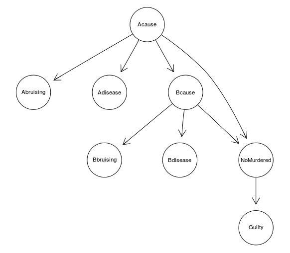
| Node | Corresponding RV |
|---|---|
| Abruising | Was bruising found on child A? |
| Bbruising | Was bruising found on child B? |
| Acause | Was the cause of death of child A natural? |
| Bcause | Was the cause of death of child B natural? |
| Adisease | Were any sings of potentially lethal disease found in child A? |
| Bdisease | Were any sings of potentially lethal disease found in child B? |
| NoMurdered | How many children were murdered? |
| Guilty | Is Sally Clark responsible for any of these deaths? |
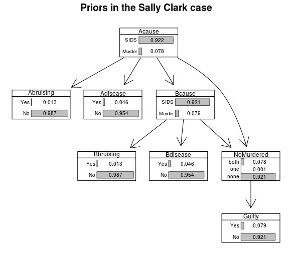
Now, let’s add CPTs and graph the marginal probabilites prior to obtaining any evidence:
#CPTs as used in Fenton & al.

AcauseProb <-prior.CPT("Acause","SIDS","Murder",0.921659)
AbruisingProb <- single.CPT("Abruising","Acause","Yes","No","SIDS","Murder",0.01,0.05)
AdiseaseProb <- single.CPT("Adisease","Acause","Yes","No","SIDS","Murder",0.05,0.001)
BbruisingProb <- single.CPT("Bbruising","Bcause","Yes","No","SIDS","Murder",0.01,0.05)
BdiseaseProb <- single.CPT("Bdisease","Bcause","Yes","No","SIDS","Murder",0.05,0.001)
BcauseProb <- single.CPT("Bcause","Acause","SIDS","Murder","SIDS","Murder",0.9993604,1-0.9998538)

#E goes first; order: last variable through levels, second last, then first
NoMurderedProb <- array(c(0, 0, 1, 0, 1, 0, 0,1,0,1,0,0), dim = c(3, 2, 2),dimnames = list(NoMurdered = c("both","one","none"),Bcause = c("SIDS","Murder"), Acause = c("SIDS","Murder")))

#this one is definitional
GuiltyProb <-  array(c( 1,0, 1,0, 0,1), dim = c(2,3),dimnames = list(Guilty = c("Yes","No"), NoMurdered = c("both","one","none")))

# Put CPTs together
SallyClarkCPT <- list(Acause=AcauseProb,Adisease = AdiseaseProb,
                      Bcause = BcauseProb,Bdisease=BdiseaseProb,
                      Abruising = AbruisingProb,Bbruising = BbruisingProb,
                      NoMurdered = NoMurderedProb,Guilty=GuiltyProb)

# join with the DAG to get a BN
SallyClarkBN <- custom.fit(SallyClarkDAG,SallyClarkCPT)

graphviz.chart(SallyClarkBN,type="barprob")
Now we can investigate the impact of subsequent developments.
#convert to a junction tree
SallyClarkJN <- compile(as.grain(SallyClarkBN))

#the prior of guilt
querygrain(SallyClarkJN, node = "Guilty")
## $Guilty
## Guilty
##        Yes         No
## 0.07893049 0.92106951
#say bruising was found on child A:
SallyClarkJNbra <- setEvidence(SallyClarkJN, nodes = c("Abruising"), states = c("Yes"))
querygrain(SallyClarkJNbra, node = "Guilty")
## $Guilty
## Guilty
##       Yes        No
## 0.2986944 0.7013056
#say bruising is also found on child B:
SallyClarkJNbrab <- setEvidence(SallyClarkJN, nodes = c("Abruising","Bbruising"),
                                states = c("Yes","Yes"))
querygrain(SallyClarkJNbrab, node = "Guilty")
## $Guilty
## Guilty
##       Yes        No
## 0.6804408 0.3195592
#if no sings of disease in children:
SallyClarkJNbrabNoDisease <- setEvidence(SallyClarkJN, nodes = c("Abruising","Bbruising","Adisease","Bdisease"),
                                states = c("Yes","Yes", "No", "No"))
querygrain(SallyClarkJNbrabNoDisease, node = "Guilty")
## $Guilty
## Guilty
## Yes No
## 0.7018889 0.2981111
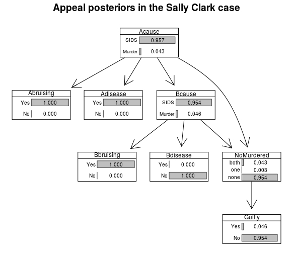
Quite crucially, the succesful appeal relied on the evidence of disease for Child A, and once we incorporate this evidence, we obtain the following situation:
``` r
# disease in Child A
SallyClarkJNdiseaseA <- setEvidence(SallyClarkJN, nodes = c("Abruising","Bbruising","Adisease","Bdisease"), states = c("Yes","Yes", "Yes", "No"))
querygrain(SallyClarkJNdiseaseA, node = "Guilty")
```
## $Guilty
## Guilty
## Yes No
## 0.04587482 0.95412518
The probability of guilt drops to 4.59% and the resulting marginals are as follows:
# disease in Child A
SallyClarkJNdiseaseA <- setEvidence(SallyClarkJN, nodes = c("Abruising","Bbruising","Adisease","Bdisease"), states = c("Yes","Yes", "Yes", "No"))
querygrain(SallyClarkJNdiseaseA, node = "Guilty")
## $Guilty
## Guilty
##        Yes         No
## 0.04587482 0.95412518
SallyClarkFinalBN <- as.bn.fit(SallyClarkJNdiseaseA, including.evidence = TRUE)
graphviz.chart(SallyClarkFinalBN,type="barprob", scale = c(0.7,1.3))
What would happen if signs of disease were present on Child B?
SallyClarkJNdiseaseAB <- setEvidence(SallyClarkJN, nodes = c("Abruising","Bbruising","Adisease","Bdisease"), states = c("Yes","Yes", "Yes", "Yes"))
querygrain(SallyClarkJNdiseaseAB, node = "Guilty")
## $Guilty
## Guilty
##          Yes           No
## 0.0009148263 0.9990851737
Scenarios with BNs
Arguably, in legal contexts, it is not only individual pieces of evidence that need to be assessed, but also whole scenarios which make sense of all them and connect them to hypotheses about what happened and about the guilt of the suspect. A method for developing BNs for that purpose is has been provided in the works of researchers such as Shen, Keppens, Aitken, Schafer, Lee , Bex and quite a few others (see our SEP entry for references).
Start with collecting all relevant scenarios and deciding which guilt hypothesis node they support (making sure you use binary guilt nodes are either the same, or exclude each other). For each state and event mentioned in a scenario, and for each piece of evidence, include a binary node in the BN and connect them as appropriate.
Next, add a binary scenario node as a parent of all the elements of the narration, and a guilt hypothesis node as its child. This is the Scenario idiom.
The CPT for the scenario node is such that the probability of each of its child is 1 given the scenario node takes value true, and equals the prior probability of a given node if its \textrm{false}. The CPT for the guilt node is such that it takes value true if the scenario node is true and false otherwise. A simple example might look like this.
ScenarioBN <- model2network("[Scenario][State/event 1|Scenario][State/event 2|Scenario:State/event 1][State/event 3|Scenario:State/event 2][Guilt|Scenario][Evidence 1|State/event 1][Evidence 2|State/event 2][Evidence 3|State/event 3]")
graphviz.plot(ScenarioBN)
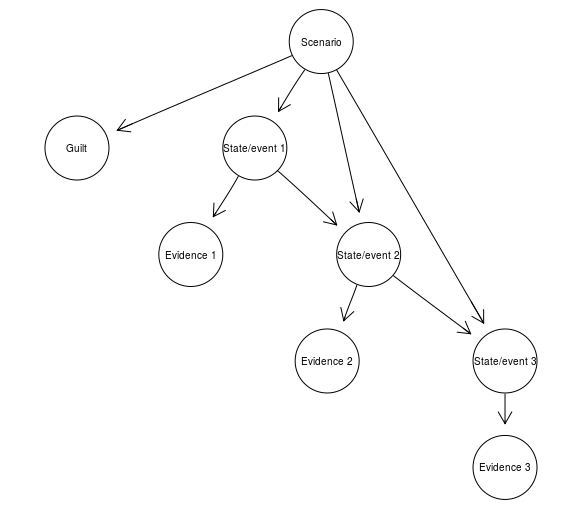
The advantage of adding a scenario node, supposedly, is that it keeps a narration as a coherent whole, so that now increasing the probability of one elements of the narration propagates to increase the probability of other elements of the scenario, and that it makes it possible to built a larger BN in which the interaction of multiple different narrations can be studied. WE find this debatable, but a deeper discussion is beyond the scope of what we’re doing now.
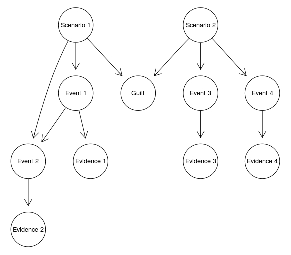
To merge two scenarios, first put their corresponding BNs together. Then, if some of the nodes in the scenarios are identical, replace them with a single node (including the guilt hypothesis node), and for any nodes which exclude each other add a constraint node:
constraint <- model2network("[Constraint|Node 1:Node 2][Node 1][Node 2]")
with values allowed and not allowed, setting the CPT such that the node takes value 1 just in case exatly one of the nodes takes value true and 0 otherwise.
The merged scenarios might look like this:
ScenarioMerged <- model2network("[Scenario 1][Scenario 2][Event 1|Scenario 1][Event 2|Scenario 1:Event 1][Event 3|Scenario 2][Event 4|Scenario 2][Guilt|Scenario 1:Scenario 2][Evidence 1|Event 1][Evidence 2|Event 2][Evidence 3|Event 3][Evidence 4|Event 4]")
graphviz.plot(ScenarioMerged)
That’s pretty much it, at least for now. An interested reader might take a look at a bunch of neat arguments related to the simplicity obtained by the use of BNs, below.
Mathy details
Probabilistic background
While Bayes’s Theorem is of immense use when it comes to calculating various conditional probabilities, if we’re interested in the interaction of multiple hypotheses at various levels and multiple pieces of evidence, calculations quickly become inconvenient, to say the least. Moreover, if such considerations are to be presented to a fact-finder, it is rather unlikely that they would be transparent and easily understood. Luckily, a tool exist to make such tasks easier. Bayesian networks (BNs) can be used for a fairly transparent and computationally more manageable evalation and presentation of the interaction of multiple pieces of evidence and hypotheses. We’ll start with a general presentation of BNs, and then go over a few main methods of employing BNs in presentation, aggregation and evaluation of evidence in legal fact-finding.
A random variable (RV) $X$ is a function from the elements of a sample space into $\mathbb{R}$, the set of real numbers. For instance, if our sample space is the set of all potential outcomes of tossing a fair coin four times (each such outcome can be represented as a sequence, for instance $HHHT$, or $HTHT$), $X$ can be the number of heads among the tosses.
Given a probability measure $P$, two events $A$ and $B$ are conditionally independent given another event $C$, $I_{P}(A,B\vert C)$, just in case $P(A\wedge B\vert C) = P(A\vert C)P(B \vert C)$. Conditional and unconditional independence don’t have to coincide. If you toss twice a coin which is fair with probability $\frac{1}{2}$, and $\frac{3}{4}$ biased towards heads with probability $\frac{1}{2}$, the result of the second toss is not independent of the first one. After all, if the first result is heads, this increases the probability that the coin is biased, and so increases the probability of heads in the second toss. On the other hand, conditionally on knowledge whether the coin is fair, the results are independent. If the coin is fair, the probability of heads in the second toss is $\frac{1}{2}$ and if the coin is biased, it is $\frac{3}{4}$, no matter what the first result was. And in the opposite direction, indepedence can disappear when we condition. Say I have two friends, Alice and Peter, who call me regularly, but they decide to do so independently. Then, whether they call in five minutes is independent. Now, suppose the phone rings. Conditional on the phone ringing, I know that if it isn’t Alice, it’s Peter, and so the identities of the callers are no longer independent.
Two RVs $X$ and $Y$ are conditionally independent given another RV $Z$, $I_{P}(X,Y\vert Z)$ just in case for any combination of values of these RVs $x,y,z$ it is the case that $I_{P}(X=x \wedge Y=y \vert Z=z)$ (notice: $X,Y$ and $Z$ are RVs, while $x,y$ and $z$ are some particular values they can take). The notion naturally generalizes to sets of RVs. Often, instead of saying things like $P(X_1 = x_1\wedge Y_5=y_5 \vert Z_3=z_3)$ we’ll rather say $P(x_1,y_5\vert z_3)$.
Now, if we have $n$ RVs, even if we assume for simplicity that they’re binary (that is, they can take only one of two values), there are $2^n$ possible combinations of values they could take, and so a direct description of a probability measure for them would require $2^n-1$ numbers. This would be a highly unfeasible method of specifying a probability distribution for a set of random variables.
Moreover, even if we had specified the joint probability distribution for all our combinations of values of Rvs $X, Y, Z$, using it wouldn’t be the most efficient way of calculating conditional probabilities or the probability that a certain selected RV takes a certain particular value. For instance, we would have to rely on:
\[P(x_1\vert y_1) = \frac{P(x_1,y_1)}{P(y_1)} = \frac{\sum_{i}P(x_1,y_1,Z=z_i)}{ \sum_{i,j}P(X=x_j,y_1,Z=z_i)}\]in which calculations we’d have to travel through all possible values of $Z$ and $X$ – this would become even less feasible as the number of RVs and their possible values increase. With 100 binary RVs we’d need $2^{99}$ terms in the sum in the denominator, so it seems that to be able to calculate a single conditional probability we’d have to elicit quite a few unconditional ones.
Relation between BNs and probabilistic measures
A quantitative BN (further on, simply BN) is a DAG with CPTs, and we say that it represents a probabilistic measure $\mathsf{P} $ quantitatively just in case they are compatible, and $\mathsf{P} $ agrees with its assignment of CPTs. It can be shown that any quantitative BN represents a unique probabilistic measure. However, any probabilistic measure can be represented by multiple BNs.
Here’s a sketch of the argument for the last claim above, if you’re interested. Skip this passage if you aren’t. Take any permutation of the RVs under consideration, obtaining $X_1, \dots, X_k$. For each $i$ find a minimal subset $P_i$ such that $I_{\mathsf{P} {}}({X_1,\dots,x_{i-1}},X_i\vert P_i)$ — that is, a minimal set of RVs which are earlier in the squence, which makes $X_i$ independent of all the (other) RVs which are earlier in the squence. Such a set always exists, in the worst-case scenario, it is the set of all $X_1,\dots,X_{i-1}$. Next, make $P_i$ the parents of $X_i$ in the DAG and copy the values of $\mathsf{P} $ into the CPTs.
The edges in a BN, intuitively, are meant to capture direct influence between RVs. The role that such direct influence plays is that in a BN any RV is conditionaly independent of its nondescentants (including ancestors), given its parents. If this is the case for a given probabilistic measure $\mathsf{P}$ and a given DAG $\mathsf{G}$, we say that $\mathsf{P}$ is compatible with $\mathsf{G}$, or that it satisfies the Markov condition.
Now, why is dealing with BNs simpler? Here’s a rough explanation. The chain rule tells us that $\mathsf{P}(A\wedge B) = \mathsf{P}(A\vert B)\mathsf{P}(B)$. Its application to RVs (say the RVs in G are $X_1,\dots X_n$) yields:
\[\mathsf{P}(x_1,\cdots,x_n) = \mathsf{P}(x_n\vert x_1,\cdots,x_{n-1})\times \\ \mathsf{P}(x_{n-1}\vert x_1,\cdots,x_{n-2})\times \\ \nonumber \times \cdots \times \mathsf{P}(x_2 \vert x_1) \mathsf{P}(x_1)\]So, if $\mathsf{P}$ is compatible with $\mathsf{G}$, we don’t have to represent it directly by listing all the $2^n-1$ values. Instead, the joint probability $\mathsf{P}(X_1\dots,X_n)$ (note: this is really an assignment of probability values to all possible combinations of the values of these RVs), can be represented using the conditional probabilities on the right-hand side of the formula, and moreover, for each conditional probability of an RVs $X$ given some other RVs, non-parents of $X$ can be removed from the condition, since RVs are independent of them.
D-separation and independence
An explanation how independence is connected with the structure of a DAG. A reader familiar with the notion of d-separation can safely skip this section.
Since information about which RVs are independent is important (they can be dropped in calculations), so is identifying the graphical counterpart of probabilistic independence, the so-called d-separation. We say that two RVs, $X$ and $Y$, are d-separated given a set of RVs $\mathsf{Z}$ — $D(X,Y\vert \mathsf{Z})$ — iff for every undirected path from $X$ to $Y$ there is a node $Z’$ on the path such that either:
-
$Z’ \in \mathsf{Z}$ and there is a serial connection, $\rightarrow Z’ \rightarrow$, on the path,
-
$Z’\in \mathsf{Z}$ and there is a diverging connection, $\leftarrow Z’ \rightarrow $, on the path,
-
There is a connection $\rightarrow Z’ \leftarrow$ on the path, and neither $Z’$ nor its descendants are in $\mathsf{Z}$.
Finally, two sets of RVs, $\mathsf{X}$ and $\mathsf{Y}$ are d-separated given $\mathsf{Z}$ if every node in $\mathsf{X}$ is d-separated from every node in $\mathsf{Y}$ given $\mathsf{Z}$.
With serial connection, for instance, if:
| RV | Proposition |
|---|---|
| $G$ | The suspect is guilty. |
| $B$ | The blood stain comes from the suspect. |
| $M$ | The crime scene stain and the suspect’s blood share their DNA profile. |
We naturally would like to have the connection $G \rightarrow B \rightarrow M$. If we don’t know whether $B$ holds, $G$ seems to have an indirect impact on the probability of $M$. Yet, once we find out that $B$ is true, we expect the profile match, and whether $G$ holds has no further impact on the probability of $M$.
The case of diverging connections has already been discussed when we talked about idependence. Whether a coin is fair, $F$, or not has impact on the result of the first toss, $H1$, and the result of the second toss, $H2$, and as long as we don’t know whether $F$, $H1$ increases the probability of $H2$. So $H1 \leftarrow F \rightarrow H2$ seems to be appropriate. Once we know that $F$, though, $H1$ and $H2$ become independent.
For converging connections, let $G$ and $B$ be as above, and let:
| RV | Proposition |
|---|---|
| $O$ | The crime scene stain comes from the offender. |
Both $G$ and $O$ influence $B$. If he’s guilty, it’s more likely that the blood stain comes from him, and if the blood crime stain comes from the offender it is more likely to come from the suspect (for instance, more so than if it comes from the victim). Moreover, $G$ and $O$ seem independent – whether the suspect is guilty doesn’t have any bearing on whether the stain comes from the offender. Thus, a converging connection $G\rightarrow B \leftarrow O$ seem appropriate. However, if you do find out that $B$ is true, that the stain comes from the suspect, whether the crime stain comes from the offender becomes relevant for whether the suspect is guilty.
Coming back to the cancer example, ${SH, S}$ d-separates $PS$ from $C$, because of the first condition used in the definition of d-separation. ${PS}$ d-esparates $SH$ from $S$. There are two paths between these RVs. The top one goes through $PS$ and fits our second condition. The bottom one goes through $C$ and fits the third condition. On the other hand, ${PS, C}$ does not d-separate $SH$ from $S$. While there is a path throuth $PS$ which satisfies the second condition, the other path contains a connection converging on $C$, and yet $C$ is in the set on which we’re conditioning.
One important reason why d-separation matters is that it can be proven that if two sets of RVs are d-separated given a third one, then they are independent given the third one, for any probabilistic measures compatible with a given DAG. Interestingly, lack of d-separation doesn’t entail dependence for any compatible probabilistic measure. Rather, it only allows for it: if RVs are d-separated, there is at least one probabilistic measure according to which they are independent. So, at least, no false independence can be inferred from the DAG, and all the dependencies are built into it.
Whence (relative) simplicity?
This is a somewhat more technical explanation of how BNs help in reducing complexity. An uninterested reader can skip it.
First, the chain rule tells us that $P(A\wedge B) = P(A\vert B)P(B)$. Its application to RVs (say the RVs in G are $X_1,\dots X_n$) yields:
\[P(x_1,\cdots,x_n) = P(x_n\vert x_1,\cdots,x_{n-1})\times \\ = P(x_{n-1}\vert x_1,\cdots,x_{n-2})\times \\ \times \cdots \times P(x_2 \vert x_1) P(x_1)\]So, if $P$ is compatible with $\mathsf{G}$, we don’t have to represent it directly by listing all the $2^n-1$ values. Instead, the joint probability $P(X_1\dots,X_n)$ (note: this is really an assignment of probability values to all possible combinations of the values of these RVs), can be represented using the conditional probabilities on the right-hand side, and moreover, for each conditional probability of an RVs $X$ given some other RVs, non-parents of $X$ can be removed from the condition, since RVs are independent of them. Let’s slow down and take a look at the argument. Pick an ancestral ordering $X_1, \dots, X_n$, of the RVs, that is, an ordering in which if $Z$ is a descendant of $X$, $Z$ follows $Y$ in the ordering. Take any selection of values of these variables, $x_1, \dots, x_n$. Let $\mathsf{pa_i}$ be the set containing all the values of the parents of $X_i$ that belong to this sequence. Since this is an ancestral ordering, the parents have to occur before $x_i$. We need to prove
\[P(x_n, x_{n-1}, \dots, x_1) = P(x_n\vert \mathsf{pa_n})P(x_{n-1}\vert \mathsf{pa_{n-1}})\cdots P(x_1)\]We prove it by induction on the length of the sequence. The basic case comes for free. Now assume:
\[P(x_i, x_{i-1}, \dots, x_1 = P(x_i\vert \mathsf{pa_i})P(x_{i-1}\vert \mathsf{pa_{i-1}})\cdots P(x_1)\]we need to show:
\[P(x_{i+1}, x_{i}, \dots, x_1) = P(x_{i+1}\vert \mathsf{pa_{i+1}})P(x_{i}\vert \mathsf{pa_{i}})\cdots P(x_1)\label{eq:markoproof3}\]One option is that $P(x_i,x_{i-1},\dots,x)=0$. Then, also $P(x_{i+1}, x_{i}, \dots, x_1)=0$, and by the induction hypothesis, there is a $1\leq k\leq i$ such that $P(x_k\vert \mathsf{pa_k})=0$, and so also the right-hand side equals 0 and so the claim holds.
Another option is that $P(x_i,x_{i-1},\dots,x)\neq 0$. Then we reason:
\[P(x_{i+1}, x_{i}, \dots, x_1) = P(x_{i+1}\vert x_i, \dots, x_1) P(x_i, \dots, x_1)\\ = P(x_{i+1}\vert \mathsf{pa_{i+1}}) P(x_i, \dots, x_1)\\ = P(x_{i+1}\vert \mathsf{pa_{i+1}}) P(x_{i}\vert \mathsf{pa_{i}})\cdots P(x_1)\]The first step is by the chain rule. The second is by the Markov condition and the fact that we employed an ancestral ordering. The third one uses an identity we already obtained. This ends the proof.
Now, why does the product of CPTs yield a joint probability distribution satisfying the Markov condition, if we’re dealing with discrete RVs?
The argument for the discrete case is as follows. Fix an ancestral ordering of the RVs and definite joint probability in terms of the conditional probabilities determined by the CPTs as we already did. We need to show it indeed is a probabilistic measure. Since the conditional probabilities are between 0 and 1, clearly so is their product. Then we need to show that the sum of $P(x_1,x_2,\dots,x_n)$ for all combinations of values of $X_1,X_2,\dots, X_n$ is 1. This can be shown by moving summation symbols around, the calculations start as follows:
\[\sum_{x_1,\dots,x_n}P(x_1,\dots, x_n) = \\ = \sum_{x_1,\dots,x_n} P(x_n\vert \mathsf{pa_n})P(x_{n-1}\vert \mathsf{pa_{n-1}})\cdots P(x_1)\\ = \sum_{x_1,\dots,x_{n-1}}\left[\sum_{x_n}P(x_n\vert \mathsf{pa_n})\right] P(x_{n-1}\vert \mathsf{pa_{n-1}})\cdots P(x_1)\\ = \sum_{x_1,\dots,x_{n-1}}P(x_1,\dots, x_{n-1})\left[1\right] \dots P(x_{n-1}\vert \mathsf{pa_{n-1}})\cdots P(x_1)\\\]when we continue this way, all the factors reduce to 1.
To show that the Markov condition holds in the resulting joint distribution we have to show that for any $x_k$ we have $P(x_k\vert \mathsf{nd_k})= P(x_k \vert \mathsf{pa_k})$, where $nd_k$ is any combination of values for all the nondescendants of $X_k$, $\mathsf{ND_k}$. So take any $k$, order the nodes so that all and only the nondescendants of $X_k$ precede it. Let $\widehat{x}_k,\widehat{nd}_k$ be some particular values of $X_k$ and $\mathsf{ND_k}$. $\mathsf{d_k}$ ranges over combinations of values of the descendants of $X_K$. The reasoning goes:
\[P(\widehat{x}_k\vert \widehat{nd}_k) = \frac{P(\widehat{x}_k,\widehat{nd}_k)}{P(\widehat{nd}_k)}\\ = \frac{\sum_{\mathsf{d_k}}P(\widehat{x}_1, \dots,\widehat{x}_k,x_{k+1},\dots, x_n)}{ \sum_{\mathsf{d_k}\cup\{x_k\}}P(\widehat{x}_1, \dots,\widehat{x}_{k-1},x_{k},\dots, x_n)} \\ = \frac{\sum_{\mathsf{d_k}}P(x_n\vert \mathsf{pa_n})\cdots P(x_{k+1}\vert \mathsf{pa_{k+1}})P(\widehat{x}_{k}\vert \mathsf{\widehat{pa}_{k}})\cdots P(\widehat{x}_1) }{ \sum_{\mathsf{d_k}\cup\{x_k\}}P(x_n\vert \mathsf{pa_n})\cdots P(x_{k}\vert \mathsf{pa_{k}})P(\widehat{x}_{k-1} \vert \mathsf{\widehat{pa}_{k-1}})\cdots P(\widehat{x}_1) } \\ = \frac{P(\widehat{x}_{k} \vert \mathsf{\widehat{pa}_{k}}) \cdots P(\widehat{x}_1)\sum_{\mathsf{d_k}}P(x_n\vert \mathsf{pa_n})\cdots P(x_{k+1}\vert \mathsf{pa_{k+1}}) }{ P(\widehat{x}_{k-1} \vert \mathsf{\widehat{pa}_{k-1}})\cdots P(\widehat{x}_1)\sum_{\mathsf{d_k}\cup\{x_k\}}P(x_n\vert \mathsf{pa_n})\cdots P(x_{k}\vert \mathsf{pa_{k}}) }\]Now, the sums in the fractions sum both to 1 (for reasons clear from the previous step of the proof), and
\[P(\widehat{x}_{k-1} \vert \mathsf{\widehat{pa}_{k-1}} )\cdots P(\widehat{x}_1)\]are both in the numerator and the denominator, so we are left with
\[P(\widehat{x}_{k} \vert \mathsf{\widehat{pa}_{k}})\]as desired.
The chain rule tells us that $\mathsf{P}(A\wedge B) = \mathsf{P}(A\vert B)\mathsf{P}(B)$. Its application to RVs (say the RVs in G are $X_1,\dots X_n$) yields:
\[\mathsf{P}(x_1,\cdots,x_n) = \mathsf{P}(x_n\vert x_1,\cdots,x_{n-1})\times \\ \mathsf{P}(x_{n-1}\vert x_1,\cdots,x_{n-2})\times \\ \times \cdots \times \mathsf{P}(x_2 \vert x_1) \mathsf{P}(x_1)\]As we already pointed out, the joint probability $\mathsf{P}(X_1\dots,X_n)$ can be represented using the conditional probabilities on the right-hand side of the formula above, and moreover, for each conditional probability of an RVs $X$ given some other RVs, non-parents of $X$ can be removed from the condition, since RVs are independent of them. Let’s slow down and take a look at the argument. Pick an ancestral ordering $X_1, \dots, X_n$, of the RVs, that is, an ordering in which if $Z$ is a descendant of $X$, $Z$ follows $Y$ in the ordering. Take any selection of values of these variables, $x_1, \dots, x_n$. Let $\mathsf{pa_i}$ be the set cotaining all the values of the parents of $X_i$ that belong to this sequence. Since this is an ancestral ordering, the parents have to occur before $x_i$. We need to prove:
\[\mathsf{P}(x_n, x_{n-1}, \dots, x_1) = \mathsf{P}(x_n\vert \mathsf{pa_n})\mathsf{P}(x_{n-1}\vert \mathsf{pa_{n-1}})\cdots \mathsf{P}(x_1)\label{eq:markoproof1}\]We prove it by induction on the length of the sequence. The basic case comes for free. Now assume:
\[\mathsf{P}(x_i, x_{i-1}, \dots, x_1 = \mathsf{P}(x_i\vert \mathsf{pa_i})\mathsf{P}(x_{i-1}\vert \mathsf{pa_{i-1}})\cdots \mathsf{P}(x_1)\label{eq:markoproof2}\]we need to show:
\[\mathsf{P}(x_{i+1}, x_{i}, \dots, x_1) = \mathsf{P}(x_{i+1}\vert \mathsf{pa_{i+1}})\mathsf{P}(x_{i}\vert \mathsf{pa_{i}})\cdots \mathsf{P}(x_1)\]One option is that $\mathsf{P}(x_i,x_{i-1},\dots,x)=0$. Then, also $\mathsf{P}(x_{i+1}, x_{i}, \dots, x_1)=0$, and by the induction hypothesis, there is a $1\leq k\leq i$ such that $\mathsf{P}(x_k\vert \mathsf{pa_k})=0$, and so also the right-hand side equals 0 and so the claim holds.
Another option is that $\mathsf{P}(x_i,x_{i-1},\dots,x)\neq 0$. Then we reason:
\[\mathsf{P}(x_{i+1}, x_{i}, \dots, x_1) = \mathsf{P}(x_{i+1}\vert x_i, \dots, x_1) \mathsf{P}(x_i, \dots, x_1)\\ = \mathsf{P}(x_{i+1}\vert \mathsf{pa_{i+1}}) \mathsf{P}(x_i, \dots, x_1)\\ = \mathsf{P}(x_{i+1}\vert \mathsf{pa_{i+1}}) \mathsf{P}(x_{i}\vert \mathsf{pa_{i}})\cdots \mathsf{P}(x_1)\]The first step is by the chain rule. The second is by the Markov condition and the fact that we employed an ancestral ordering. The third one uses \eqref{eq:markoproof2}. This ends the proof.
Computation in BNs is easier than direct calculations, but this doesn’t mean it’s easy. In general, the problem is NP-hard, but efficient algorithms exist for exact calculations and for Monte Carlo estimations (which employ simulations) for certain groups of BNs. More importantly, humans are decent at identifying features of reality that seem important for a given problem, but terrible at aggregating the information they have about all of them. This is where BNs come to the rescue: a human reasoner constructs a DAG according to their theoretical preconceptions, separately specifies what they think about parent nodes and their children, and automated calculation with a BN does the rest of the job.