Probably?
(Mainly) bayesian data analysis with a philosophical twist
False positives in DNA identification 3
Hopefully, having convinced the reader that the false positive probability is non-negligible, I can now move to a probabilistic approach to the impact such probability can have on the value of evidence. Since I will use the likelihood ratio, a fairly standard measure of evidential strength, I first explain this notion, then explain one relevant formula and its derivation, leaving another perspective to another post.
The likelihood ratio is a comparative measure of whether evidence $E$ supports a hypothesis $H$ more than a competing hypothesis $H’$, in symbols: \begin{align} \label{eq:LR} \mathsf{LR}(E,H,H’) & = \frac{\mathsf{P}(E \vert H)}{\mathsf{P}(E \vert H’)}. \end{align}
If the evidence supports $H$ more than $H’$, the ratio would be above one, and if the evidence supports $H’$ more than $H$, the ratio would be below one. So, support levels correspond to deviations from one. The greater the likelihood ratio (for values above one), the stronger the evidence in favor of $H$ as contrasted with $H’$. The smaller the likelihood ratio (for values below one), the stronger the evidence in favor of the competing hypothesis $H’$ as contrasted with $H$.
Experts sometimes testify by offering the likelihood ratio as a measure of the strength of the evidence. An expert, for instance, may testify that the blood-staining on the jacket of the defendant is ten times more likely to be seen if the wearer of the jacket hit the victim (prosecutor’s hypothesis) rather than if he did not (defense’s hypothesis) (CGG Aitken, Roberts, & Jackson, 2010, p. 38). Experts are typically advised not to comment on the posterior odds given the evidence. As this formulation of the Bayes’s theorem makes clear, an assessment of the posterior odds will require a judgment about the prior odds, and the latter lies beyond the competence of an expert. A prominent forensic scientist recommends that experts `not trespass on the province of the jury by commenting directly on the accused’s guilt or innocence, and should generally confine their testimony to presenting the likelihood of their evidence under competing propositions’ (CGG Aitken et al., 2010, p. 42).
Now, let us follow Colin Aitken, Taroni, & Thompson (2003) in investigating its impact on the likelihood ratio of the DNA match. We just add a bit more details to the derivation they present for the sake of clarity. For simplicity, we still assume that the false negative probability is 0, that is, that if the match is real, it will be reported with certainty. We abbreviate:
| $S$ | The specimen comes from the suspect. |
| $R$ | A match is reported. |
| $M$ | There is a true match. |
The formula we will end up with is:
\begin{align} \mathsf{LR}(R, S, \neg S) & = \frac{1}{RMP + [ FPP \times (1-RMP)]} \end{align}
where RMP stands for the random match probability and FPP for the false positive probability. We will assume that whether a (lack of) match is reported is independent of whether it is coincidental,
\begin{align} \mathsf{P}(R \vert M \wedge S) = \mathsf{P}(R \vert M \wedge \neg S) = \mathsf{P}(R \vert M)\end{align} \begin{align} \mathsf{P}(R \vert \neg M \wedge S) = \mathsf{P}(R \vert\neg M \wedge \neg S) = \mathsf{P}(R \vert \neg M) \end{align} that the probability of true match if the suspect is a source is 1, \begin{align} \mathsf{P}(M\vert S) = 1 \,\,\, \mbox{ so also } \,\,\, \mathsf{P}(\neg M \vert S)=0, \end{align} and that the probability that a true match is reported, \begin{align}\mathsf{P}(R \vert M) & = 1.\end{align}
The formula we will end up with is:
\begin{align} \mathsf{LR}(R, S, \neg S) = \frac{1}{RMP + [ FPP \times (1-RMP)]} \end{align} where RMP stands for the random match probability and FPP for the false positive probability. We will assume that whether a (lack of) match is reported is independent of whether it is coincidental, \begin{align} \mathsf{P}(R \vert M \wedge S) = \mathsf{P}(R \vert M \wedge \neg S) = \mathsf{P}(R \vert M) \end{align} \begin{align} \mathsf{P}(R \vert \neg M \wedge S) = \mathsf{P}(R \vert\neg M \wedge \neg S) = \mathsf{P}(R \vert \neg M), \end{align} that the probability of true match if the suspect is a source is 1, \begin{align} \mathsf{P}(M\vert S) = 1 \,\,\, \mbox{ so also } \,\,\, \mathsf{P}()\neg M \vert S)=0, \end{align} and that the probability that a true match is reported, \begin{align} \mathsf{P}(R \vert M) = 1. \end{align}
Here, for simplicity we take the probability of a false negative to be null; in fact, some of the reasons for taking false positives seriously are also reasons to take false negatives seriously, but let’s deal with one problem at a time (and in the end, the impact of a false positive risk will be clear from the way the formula will be derived). Now, let us rewrite the numerator of the LR by extending the conversation, rewriting the probabilities of conjunctions in terms of conditional probability and simplifying:
\begin{align} \mathsf{P}(R\vert S) = \frac{\mathsf{P}(R\wedge S)}{\mathsf{P}(S)} = \frac{\mathsf{P}(R \wedge M \wedge S) + \mathsf{P}(R \wedge \neg M \wedge S)} {\mathsf{P}(S)} \end{align} \begin{align} = \frac{\mathsf{P}(R \vert M \wedge S)\mathsf{P}(M \vert S)\mathsf{P}(S) + \mathsf{P}(R \vert \neg M \wedge S)\mathsf{P}()\neg M \vert S)\mathsf{P}(S)} {\mathsf{P}(S)} \end{align}\begin{align} = \mathsf{P}(R \vert M \wedge S)\mathsf{P}(M \vert S) + \mathsf{P}(R \vert \neg M \wedge S)\mathsf{P}()\neg M \vert S) \end{align}
Analogously, we can rewrite the denominator: \begin{align} \mathsf{P}(R \vert \neg S) = \mathsf{P}(R \vert M \wedge \neg S)\mathsf{P}(M \vert \neg S) + \mathsf{P}(R \vert \neg M \wedge \neg S)\mathsf{P}(\neg M \vert \neg S) \end{align}
Putting these together, we have that: \begin{align} \mathsf{LR}(R,S, \neg S) = \frac{\mathsf{P}(R \vert M \wedge S)\mathsf{P}(M \vert S) + \mathsf{P}(R \vert \neg M \wedge S) \mathsf{P}(\neg M \vert S)} {\mathsf{P}(R \vert M \wedge \neg S)\mathsf{P}(M \vert \neg S) + \mathsf{P}(R \vert \neg M \wedge \neg S)\mathsf{P}(\neg M \vert \neg S)} \end{align} Now, apply one of the identities in four places: \begin{align} \mathsf{LR}(R,S, \neg S) = \frac{ \mathsf{P}(R \vert M)\mathsf{P}(M \vert S) + \mathsf{P}(R \vert \neg M)\mathsf{P}(\neg M \vert S) }{ \mathsf{P}(R \vert M )\mathsf{P}(M \vert \neg S) + \mathsf{P}(R \vert \neg M)\mathsf{P}(\neg M \vert \neg S) } \end{align} Then, rewrite the numerator: \begin{align} \mathsf{LR}(R,S, \neg S) = \frac{ \mathsf{P}(R \vert M) \times 1 + \mathsf{P}(R \vert \neg M)\times 0 }{ \mathsf{P}(R \vert M )\mathsf{P}(M \vert \neg S) + \mathsf{P}(R \vert \neg M)\mathsf{P}(\neg M \vert \neg S) } \end{align} Finally, we have: \begin{align} \mathsf{LR}(R,S, \neg S) & = \frac{1} {\mathsf{P}(R \vert M)\mathsf{P}( M \vert \neg S) + \mathsf{P}(R \vert \neg M)\mathsf{P}(\neg M \vert \neg S)} \end{align} Once we abbreviate $\mathsf{P}(M\vert \neg S)$ as RMP, $\mathsf{P}(R \vert \neg M)$ as FPP and $\mathsf{P}(\neg M \vert \neg S)$, we arrive at the desired formula.
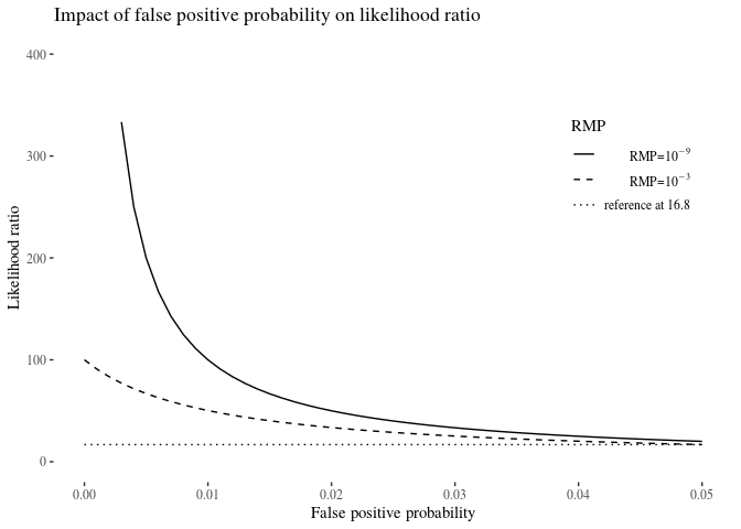
We now illustrate this impact for the range of FPP between 0 and 0.05, for two values of RMP: $10^{-9}$ (often reported in the case of two single-source samples over ten or more loci) and $10{^-3}$ (sometimes obtained by means of less discriminating tests when the comparison involves a mixed sample). The upshot is that even a small increase in FPP can lower the likelihood ratio dramatically, which is yet another reason not to ignore FPP in DNA evidence evaluation. In our illustration, we look at two pieces of DNA evidence with the two RMP rates at $1*10^8$ and $100$, respectively. If the false positive probability reaches 0.02, they fall down to $\approx 49.99$ and $\approx 33.55$, and they get fairly close to each other already at $FPP=0.05$, where they are $\approx 20$ and $\approx 16.8$.
rmp9 <- 10e-9
rmp3 <- 10e-3
fpp <- seq(0,0.05, by = 0.001)

lr9 <- 1/(rmp9 + (fpp * (1-rmp9)))
lr3 <- 1/(rmp3 + (fpp * (1-rmp3)))


fppTable <- data.frame(fpp,   lr9,  lr3, ref = rep(16.8, length(fpp)))

library(tidyr)
fppTableLong <- gather(fppTable,line,value,c(lr9,lr3,ref), factor_key=TRUE)


ggplot(fppTableLong, aes(x=fpp,y=value, lty = line))+ geom_line()+ylim(c(0,400))+
  theme_tufte()+ylim(c(0,400))+
  ylab("Likelihood ratio")+
  xlab("False positive probability")+
  scale_linetype_manual(values = c(1,2,3),labels = c(expression(paste("RMP=",10^{-9})),expression(paste("RMP=",10^{-3})),"reference at 16.8"))+
  ggtitle("Impact of false positive probability on likelihood ratio")+
  theme(legend.position = c(0.85,.7))+ labs(lty = "RMP")
Aitken, C., Roberts, P., & Jackson, G. (2010). Fundamentals of probability and statistical evidence in criminal proceedings (Practitioner Guide No. 1), Guidance for judges, lawyers, forensic scientists and expert witnesses. Royal Statistical Society’s Working Group on Statistics and the Law.
Aitken, C., Taroni, F., & Thompson, W. (2003). How the probability of a false positive affects the value of dna evidence. Journal of Forensic Science, 48(1), 1–8. https://doi.org/10.1520/jfs2001171
Written on August 19th, 2021 by Rafal Urbaniak