Signal with Mediation: SHAP, Causal SHAP, and PCI

Imagine a feature \(X\) that influences an outcome \(Y\) only through an intermediate variable \(M\): the mediation chain \(X \to M \to Y\). \(X\) never touches \(Y\) directly; it acts only by moving \(M\), which in turn moves \(Y\). This three-variable model is a demanding test for explanation methods, because any correct answer to “what caused \(Y\)?” must respect the asymmetry: \(M\) is the direct cause of \(Y\), and \(X\) only an indirect one. A trustworthy method should rank the two differently without being told to.

Most popular attribution methods fail that test. Leaning on statistical association, they tend to hand \(X\) and \(M\) the same credit for \(Y\), blind to the fact that \(X\) acts only indirectly, and they will even credit a variable for an outcome it merely predicts, scoring \(Y\) as a cause of \(X\) just because the two are correlated. This notebook lines up three methods on one Gaussian chain and grades each against the demands of the causal structure:

plain SHAP: the standard feature-attribution game;
causal SHAP: the same game with interventional (\(\mathrm{do}\)) baselines; and
PCI (Probabilistic Causal Impact): the paper’s method.

The discriminating test is D-MXY: whether a method ranks the direct cause \(M\) above the indirect cause \(X\) for \(Y\), or at least apart from it. Both SHAP variants tie the two and fail it, whereas PCI separates them on structure alone, and adding the mediator as a witness sharpens the separation further.

This notebook reproduces every number in the Signal with Mediation example and uses the desiderata names (D-XY, D-MY, D-MXY, …) exactly as stated there; the derivations it refers to are all reproduced in the code cells here, so it stands on its own.

Outline

Model and setup
The seven desiderata
Optimal predictors (the models SHAP explains)
Plain SHAP
Causal SHAP
PCI without witnesses
PCI with witnesses
The desiderata scorecard
General analytic forms for any instance
Instance 2: the baseline, where SHAP collapses to zero
Instance 3: a counter-responsible \(X\)
Three-instance comparison

1. Model and setup

The generative model is a linear chain \(X \to M \to Y\) with additive Gaussian noise: \(X\) emits a signal, \(M\) relays it with some noise, and \(Y\) is the noisy final outcome. Because everything is jointly Gaussian, all conditional expectations are exactly linear and every quantity below has a closed form, so the example needs no approximations anywhere.

Variable	Distribution	Reading
\(X\)	\(\mathcal{N}(0.5,\; 0.25)\)	exogenous root cause
\(M\)	\(X + \varepsilon_M\), \(\varepsilon_M \sim \mathcal{N}(0,\, 0.1)\)	mediator
\(Y\)	\(M + \varepsilon_Y\), \(\varepsilon_Y \sim \mathcal{N}(0,\, 0.1)\)	outcome

One structural fact carries the rest of the notebook: \(X\) reaches \(Y\) only through \(M\) (the path \(X \to M \to Y\)), whereas \(M\) acts on \(Y\) directly. A method that respects causal structure should be able to tell these two roles apart.

The chain \(X \to M \to Y\) is drawn below; the mediator \(M\) and the outcome \(Y\) are highlighted.

[1]:

# Causal DAG for the signal-with-mediation model.
#
# Rendered with the SAME helper that generates the paper figure
# (scripts/make_example_dags.py): single source of truth, so this notebook and
# the paper never drift. The rendering is colour-blind-safe -- each role is
# encoded by SHAPE (box / hexagon / double box / dashed circle) as well as
# colour, and dashed U-circles mark the exogenous noise on each stochastic
# mechanism.
import pathlib
import sys

import matplotlib.pyplot as plt

_p = pathlib.Path.cwd()
for _ in range(8):
    if (_p / "scripts" / "make_example_dags.py").exists():
        sys.path.insert(0, str(_p))
        break
    _p = _p.parent
from scripts.make_example_dags import fig_signal  # noqa: E402

fig, ax = plt.subplots(figsize=(6.6, 4.2))
ax.axis("off")
ax.set_aspect("equal")
fig_signal(ax)
plt.show()

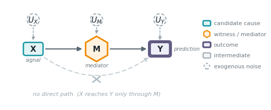
_images/signal_mediation_computations_2_0.png

Factual instance: \(x^\star = m^\star = y^\star = 1\) (Instance 1). Every variable is one above its mean of \(0.5\), so every prediction is non-trivial and all three methods return non-zero values, the simplest case to compare them on. (Sections 10–12 revisit two further instances that stress the methods.)

PCI scores one variable at a time; the variable under test is the suspect \(A\), the candidate cause whose responsibility we are scoring. PCI grades \(A\) by comparing two counterfactual worlds against the realized outcome \(y^\star\), through the causal-impact contrast \(\mathrm{ci}\) (unrelated to the CI=1 smoke-test flag introduced below):

\[\mathrm{ci}(y^s, y^n, y^\star) = \underbrace{|y^n - y^\star|}_{\text{necessity}} - \underbrace{|y^s - y^\star|}_{\text{sufficiency}}.\]

The necessity world replaces the suspect with a random redraw \(A' \sim P(A)\) and runs the model forward; a large \(|y^n - y^\star|\) means the outcome needed the suspect’s actual value. The sufficiency world restores the suspect to \(a^\star\) and runs forward with fresh noise; a small \(|y^s - y^\star|\) means the suspect on its own reliably reproduces the outcome. Subtracting the two rewards a suspect that is at once needed and enough. So \(\mathrm{ci}\) is large exactly when re-rolling the suspect moves the outcome away from \(y^\star\) (a large necessity term) while pinning it holds the outcome in place (a small sufficiency term), the two hallmarks of a genuine cause. Both worlds draw fresh exogenous noise from \(P_{\mathbf{U}}\) (the joint distribution of the noise terms, here \(\varepsilon_M\) and \(\varepsilon_Y\)), so the comparison averages the suspect’s causal role over noise realizations. A higher \(\mathrm{ci}\) means more causal responsibility.

2. Seven desiderata a correct attribution must satisfy

Before computing anything we fix the target, the conditions a good attribution method should satisfy on this chain. We grade all four methods (plain SHAP, causal SHAP, PCI without and with a witness) against the same seven desiderata, named exactly as in the paper. They refer to a generic responsibility score \(R(V \rightsquigarrow B)\), a placeholder for the number a method assigns to variable \(V\) for target \(B\), and, since SHAP can be signed, the conditions are stated on magnitudes \(\lvert R\rvert\). The seven enumerate every ordered (cause \(\to\) target) pair the chain lets us ask about, plus the discriminating comparison D-MXY.

Name	In words	Condition
D-XY	\(X\) is an (indirect) cause of \(Y\)	\(\lvert R(X\rightsquigarrow Y)\rvert > 0\)
D-MY	\(M\) is a (direct) cause of \(Y\)	\(\lvert R(M\rightsquigarrow Y)\rvert > 0\)
D-XM	\(X\) is a cause of \(M\)	\(\lvert R(X\rightsquigarrow M)\rvert > 0\)
D-YX	\(Y\) is not a cause of \(X\)	\(R(Y\rightsquigarrow X) = 0\)
D-YM	\(Y\) is not a cause of \(M\)	\(R(Y\rightsquigarrow M) = 0\)
D-MX	\(M\) is not a cause of \(X\)	\(R(M\rightsquigarrow X) = 0\)
D-MXY	\(M\) (direct) outranks \(X\) (indirect) for \(Y\)	\(\lvert R(M\rightsquigarrow Y)\rvert > \lvert R(X\rightsquigarrow Y)\rvert\)

Three groups, three jobs:

Positive (D-XY, D-MY, D-XM): the method must acknowledge a genuine causal link with a non-zero score (a negative SHAP value still counts).
Zero (D-YX, D-YM, D-MX): the method must not send credit backwards, against the arrows of the chain.
Discriminating (D-MXY): because \(X\) reaches \(Y\) only through \(M\), the direct cause \(M\) should rank strictly above the indirect cause \(X\). This is the one that separates the methods: both SHAP variants tie, PCI breaks the tie, and a witness widens the margin.

§8 assembles the full pass/fail audit: PCI passes all seven, while both SHAP variants fail the three zero desiderata and tie on D-MXY.

[2]:

import os

import numpy as np
from scipy.stats import norm

# Smoke-test mode is triggered by ``CI=1``. It shrinks the Monte Carlo sample
# size used to cross-check the closed-form PCI values. Closed-form numbers in
# the paper are unaffected; only the ``mc_*`` cross-checks get noisier.
smoke_test = "CI" in os.environ

rng = np.random.default_rng(42)
N = 10_000 if smoke_test else 2_000_000

mu_X, var_X = 0.5, 0.25
var_eM = 0.1
var_eY = 0.1
var_M = var_X + var_eM  # 0.35
var_Y = var_M + var_eY  # 0.45
cov_XM = var_X  # 0.25
cov_XY = var_X  # 0.25
cov_MY = var_M  # 0.35
mu_M = mu_X
mu_Y = mu_X
x_star, m_star, y_star = 1.0, 1.0, 1.0

print(f"Var(X)={var_X}, Var(M)={var_M}, Var(Y)={var_Y}")
print(f"Cov(X,M)={cov_XM}, Cov(X,Y)={cov_XY}, Cov(M,Y)={cov_MY}")

Var(X)=0.25, Var(M)=0.35, Var(Y)=0.44999999999999996
Cov(X,M)=0.25, Cov(X,Y)=0.25, Cov(M,Y)=0.35

3. Optimal predictors

SHAP explains a model, so we first need a predictor for each target. We use the optimal (squared-loss) predictor for each variable given the other two, which in this Gaussian model is just the conditional expectation and is exactly linear. We explain three targets in turn (\(Y\), \(M\), and \(X\)), because the desiderata ask about responsibility flowing in both causal directions (e.g. does \(Y\) wrongly get credit for \(X\)?).

\(f_Y(x, m) = m\) is exact: given \(M\), the noise \(\varepsilon_Y\) is all that separates \(M\) from \(Y\), and \(X\) adds nothing once \(M\) is known.
\(f_M(x, y)\) and \(f_X(m, y)\) are the linear least-squares predictors read off the joint Gaussian. \(f_M\) uses \(Y\) as an input even though \(Y\) is downstream of \(M\), purely because \(Y\) predicts \(M\) statistically. That backward dependence trips SHAP up later.

The cell below confirms the coefficients match the closed forms derived in Appendix B (\(f_M = 0.5X + 0.5Y\) and \(f_X = 0.5 + \tfrac{5}{7}(M - 0.5)\)).

[3]:

def f_Y(x, m):
    return m


Sigma_XY = np.array([[var_X, cov_XY], [cov_XY, var_Y]])
coeff_fM = np.array([cov_XM, cov_MY]) @ np.linalg.inv(Sigma_XY)


def f_M(x, y):
    return mu_M + coeff_fM[0] * (x - mu_X) + coeff_fM[1] * (y - mu_Y)


Sigma_MY = np.array([[var_M, cov_MY], [cov_MY, var_Y]])
coeff_fX = np.array([cov_XM, cov_XY]) @ np.linalg.inv(Sigma_MY)


def f_X(m, y):
    return mu_X + coeff_fX[0] * (m - mu_M) + coeff_fX[1] * (y - mu_Y)


print(
    f"f_M(X,Y) = 0.5 + {coeff_fM[0]:.4f}*(X-0.5) + {coeff_fM[1]:.4f}*(Y-0.5)  [expect 0.5X + 0.5Y]"
)
print(
    f"f_X(M,Y) = 0.5 + {coeff_fX[0]:.4f}*(M-0.5) + {coeff_fX[1]:.6f}*(Y-0.5)  [expect (5/7)*(M-0.5)]"
)
print(
    f"f_Y(1,1)={f_Y(1, 1):.4f}  f_M(1,1)={f_M(1, 1):.4f}  f_X(1,1)={f_X(1, 1):.4f}  [1, 1, {5 / 14 + 0.5:.4f}]"
)

f_M(X,Y) = 0.5 + 0.5000*(X-0.5) + 0.5000*(Y-0.5)  [expect 0.5X + 0.5Y]
f_X(M,Y) = 0.5 + 0.7143*(M-0.5) + 0.000000*(Y-0.5)  [expect (5/7)*(M-0.5)]
f_Y(1,1)=1.0000  f_M(1,1)=1.0000  f_X(1,1)=0.8571  [1, 1, 0.8571]

4. Plain SHAP

A Shapley value splits a prediction’s deviation from its population mean fairly among the input features, by averaging each feature’s marginal contribution over all orders in which features could be added to a coalition. To value a coalition \(S\), plain SHAP holds the features in \(S\) at their factual values and marginalises the rest using observational conditional expectations:

\[v(S) = \mathbb{E}[B \mid X_S = x_S^\star].\]

So a coalition \(S\) is worth the model’s expected output when we pin the features in \(S\) at their factual values and average the rest out from their observational distribution given \(S\).

With only \(|N| = 2\) features the Shapley formula collapses to a simple average of two marginal contributions:

\[\phi_i = \tfrac{1}{2}\bigl(v(\{i\}) - v(\emptyset)\bigr) + \tfrac{1}{2}\bigl(v(N) - v(N \setminus \{i\})\bigr).\]

Feature \(i\)’s attribution is its average marginal contribution to the prediction: the amount it adds on joining the coalition, averaged over the two orders the features can enter (alone against \(\emptyset\), or second to complete the full set \(N\)).

Because \(v(S)\) is built from observational conditionals, which are symmetric under reversal of causal direction, plain SHAP cannot tell “\(Y\) is informative about \(X\)” from “\(Y\) causes \(X\)”. We expect it to send credit backwards along the chain. The cell below computes all six (suspect \(\to\) target) values; the bracketed numbers are the paper’s targets.

[4]:

def E_cond(tmean, cov_to, var_o, oval, omean):
    return tmean + cov_to / var_o * (oval - omean)


def shapley2(vA, vB, vAB, v0):
    return 0.5 * (vA - v0) + 0.5 * (vAB - vB), 0.5 * (vB - v0) + 0.5 * (vAB - vA)


EY_X1 = E_cond(mu_Y, cov_XY, var_X, x_star, mu_X)
EX_Y1 = E_cond(mu_X, cov_XY, var_Y, y_star, mu_Y)
EM_Y1 = E_cond(mu_M, cov_MY, var_Y, y_star, mu_Y)

vY_e, vY_X, vY_M, vY_XM = mu_M, E_cond(mu_M, cov_XM, var_X, x_star, mu_X), m_star, 1.0
vM_e = f_M(mu_X, mu_Y)
vM_X = 0.5 * x_star + 0.5 * EY_X1
vM_Y = 0.5 * EX_Y1 + 0.5 * y_star
vM_XY = f_M(x_star, y_star)
vX_e = f_X(mu_M, mu_Y)
vX_M = f_X(m_star, mu_Y)
vX_Y = f_X(EM_Y1, y_star)
vX_MY = f_X(m_star, y_star)

phi_X_Y_plain, phi_M_Y_plain = shapley2(vY_X, vY_M, vY_XM, vY_e)
phi_X_M_plain, phi_Y_M_plain = shapley2(vM_X, vM_Y, vM_XY, vM_e)
phi_M_X_plain, phi_Y_X_plain = shapley2(vX_M, vX_Y, vX_MY, vX_e)

print("Plain SHAP:")
print(f"  phi_X^Y={phi_X_Y_plain:.4f} [0.250]  phi_M^Y={phi_M_Y_plain:.4f} [0.250]")
print(f"  phi_X^M={phi_X_M_plain:.4f} [0.306]  phi_Y^M={phi_Y_M_plain:.4f} [0.194]")
print(f"  phi_M^X={phi_M_X_plain:.4f} [0.219]  phi_Y^X={phi_Y_X_plain:.4f} [0.139]")

Plain SHAP:
  phi_X^Y=0.2500 [0.250]  phi_M^Y=0.2500 [0.250]
  phi_X^M=0.3056 [0.306]  phi_Y^M=0.1944 [0.194]
  phi_M^X=0.2183 [0.219]  phi_Y^X=0.1389 [0.139]

The positive direct and upstream links come out as expected: \(\phi_X^Y = \phi_M^Y = 0.250\), \(\phi_X^M = 0.306\). The failures show in the backward numbers. \(\phi_Y^X = 0.139 > 0\) says plain SHAP credits \(Y\) for \(X\), even though \(Y\) does not cause \(X\). That happens because observing \(Y{=}1\) is statistically informative about \(X{=}1\) through the chain, so the observational \(v(\{Y\})\) exceeds the baseline. Likewise \(\phi_Y^M = 0.194\) and \(\phi_M^X = 0.219\) leak backward. And \(\phi_X^Y = \phi_M^Y\) exactly: plain SHAP cannot see that \(X\) reaches \(Y\) only through \(M\), so it ties the direct and indirect causes (D-MXY fails).

5. Causal SHAP

Causal SHAP keeps the Shapley averaging and changes how a dropped feature is removed. It values a coalition under an intervention:

\[v(S) = \mathbb{E}[B \mid \mathrm{do}(X_S = x_S^\star)].\]

A feature outside the coalition is then sampled according to the causal graph: descendants of \(S\) propagate through their structural equations after the \(\mathrm{do}\), while non-descendants revert to their plain marginals (intervening on a variable cannot change something upstream of it).

The intervention severs spurious backward information flow, so we expect causal SHAP to repair the worst leak (D-YX: \(Y\) should get zero credit for \(X\)). It still cannot remove a feature that the prediction model itself uses as an input (e.g. \(Y\) inside \(f_M\)), and it cannot distinguish a direct from an indirect path, so D-YM, D-MX, and D-MXY stay broken below.

[5]:

vcY_e, vcY_X, vcY_M, vcY_XM = mu_M, 1.0, 1.0, 1.0
vcM_e = f_M(mu_X, mu_Y)
vcM_X = 0.5 * x_star + 0.5 * 1.0  # E[Y|do(X=1)] = 1
vcM_Y = 0.5 * mu_X + 0.5 * y_star  # E[X|do(Y=1)] = mu_X (breaks M->Y)
vcM_XY = f_M(x_star, y_star)
vcX_e = f_X(mu_M, mu_Y)
vcX_M = f_X(m_star, 1.0)  # do(M=1); Y coeff~0
vcX_Y = f_X(mu_M, y_star)  # do(Y=1) breaks M->Y; E[M|do(Y=1)]=mu_M
vcX_MY = f_X(m_star, y_star)

phi_X_Y_c, phi_M_Y_c = shapley2(vcY_X, vcY_M, vcY_XM, vcY_e)
phi_X_M_c, phi_Y_M_c = shapley2(vcM_X, vcM_Y, vcM_XY, vcM_e)
phi_M_X_c, phi_Y_X_c = shapley2(vcX_M, vcX_Y, vcX_MY, vcX_e)

print("Causal SHAP:")
print(f"  phi_X^Y={phi_X_Y_c:.4f} [0.250]  phi_M^Y={phi_M_Y_c:.4f} [0.250]")
print(f"  phi_X^M={phi_X_M_c:.4f} [0.375]  phi_Y^M={phi_Y_M_c:.4f} [0.125]")
print(f"  phi_M^X={phi_M_X_c:.4f} [0.357]  phi_Y^X={phi_Y_X_c:.4f} [0.000]")

Causal SHAP:
  phi_X^Y=0.2500 [0.250]  phi_M^Y=0.2500 [0.250]
  phi_X^M=0.3750 [0.375]  phi_Y^M=0.1250 [0.125]
  phi_M^X=0.3571 [0.357]  phi_Y^X=0.0000 [0.000]

The interventional fix works exactly where predicted: \(\phi_Y^X\) drops from \(0.139\) to \(0.000\) (D-YX repaired), because \(M\) is not downstream of \(Y\), so \(\mathrm{do}(Y{=}1)\) gives no leverage over \(f_X\). But the other backward scores survive: \(\phi_Y^M = 0.125\) persists because \(Y\) is an actual input of the prediction model \(f_M(X,Y)=0.5X+0.5Y\), and switching to \(\mathrm{do}\) cannot delete a feature the model uses. The fix also backfires. \(\phi_M^X\) rises from \(0.219\) to \(0.357\), because the attribution freed from \(Y\) goes to \(M\), the only visible predictor of \(X\). And \(\phi_X^Y = \phi_M^Y = 0.250\) still ties, so D-MXY remains broken. Causal SHAP fixes D-YX but not D-YM, D-MX, or D-MXY.

6. PCI without witnesses

We now switch from SHAP to PCI. Where SHAP splits a prediction’s deviation from a population mean, PCI asks a counterfactual question about the realized outcome \(b^\star\) directly: how much would it move if we intervened on the suspect? For each target \(B\) we take the suspect set \(\mathbf{S}\) to be the two input features of \(B\); we then put each input in turn in the suspect’s chair, so the same \(\mathbf{S}=\{X,M\}\) yields both \(R(X\rightsquigarrow Y)\) and \(R(M\rightsquigarrow Y)\). This section uses no witnesses (\(\mathbf{W}=\emptyset\)).

PCI averages the contrast over which subset \(\mathbf{C}\) of the suspect set we actually intervene on, with weights \(\Gamma_s\) uniform over the three non-empty subsets of \(\mathbf{S}\). Only subsets that contain the suspect \(A\) can carry its responsibility, so each of the two suspect-containing subsets (\(\mathbf{C} \ni A\)) gets weight \(\tfrac{1}{3}\). The score is the unnormalised weighted sum over just those subsets, \(R(A\rightsquigarrow B) = \sum_{\mathbf{C}\ni A}\Gamma_s(\mathbf{C})\,\bar c(\mathbf{C})\). Keeping the raw \(\tfrac{1}{3}\) weights, without renormalising to \(1\), is a deliberate design choice.

For each subset we compute the expected contrast \(\bar c = \mathbb{E}[|B^n - b^\star|] - \mathbb{E}[|B^s - b^\star|]\), the expectation of the single-draw \(\mathrm{ci}\) above, taken over fresh exogenous noise. Each expectation has a closed form through the folded-normal formula for \(\mathbb{E}|Z|\) with \(Z \sim \mathcal{N}(\mu,\sigma^2)\) (the mean of \(|Z|\) when \(Z\) is Gaussian):

the necessity expectation \(\mathbb{E}[|B^n - b^\star|]\) (suspect re-rolled),
the sufficiency expectation \(\mathbb{E}[|B^s - b^\star|]\) (suspect pinned).

A large Monte Carlo run (\(N = 2\times10^6\), or a smaller noisy run under CI=1) cross-checks each closed-form value. The next two cells set up the closed-form helper and the Monte Carlo draws; the third computes the six responsibility values.

[6]:

def E_abs_N(mu, sigma2):
    """E[|Z|] for Z ~ N(mu, sigma2). Folded-normal formula; degenerates to |mu| at sigma2=0."""
    if sigma2 <= 0:
        return abs(mu)
    sigma = np.sqrt(sigma2)
    c = mu / sigma
    return mu * (2 * norm.cdf(c) - 1) + 2 * sigma * norm.pdf(c)


# Necessity-world MC draws: alternative values for suspects, fresh exogenous noise
X_alt = rng.normal(mu_X, np.sqrt(var_X), N)
M_alt = rng.normal(mu_M, np.sqrt(var_M), N)
eM_n = rng.normal(0, np.sqrt(var_eM), N)
eY_n = rng.normal(0, np.sqrt(var_eY), N)

# Sufficiency-world MC draws: independent fresh exogenous noise
eM_s = rng.normal(0, np.sqrt(var_eM), N)
eY_s = rng.normal(0, np.sqrt(var_eY), N)

[7]:

# S = {two input features of target}, W = empty.
# Valid (C, T) pairs: C in {A} and C in {A, other}, each with Gamma weight 1/3.
# bar_c(C, T) = E[|B^n - b*|] - E[|B^s - b*|]; PCI = sum over suspect-containing pairs.
#
# DXY  S={X,M}:
#   C={X}    n: do(X=X')         Y^n = X'+eM+eY    s: do(X=x*)         Y^s = x*+eM+eY
#   C={X,M}  n: do(X=X', M=M')   Y^n = M'+eY       s: do(X=x*, M=m*)   Y^s = m*+eY

# ---- DXY ----
n_DXY_C1 = E_abs_N(mu_X - y_star, var_X + var_eM + var_eY)
s_DXY_C1 = E_abs_N(x_star - y_star, var_eM + var_eY)
n_DXY_C2 = E_abs_N(mu_M - y_star, var_M + var_eY)
s_DXY_C2 = E_abs_N(m_star - y_star, var_eY)
pci_DXY_nw = ((n_DXY_C1 - s_DXY_C1) + (n_DXY_C2 - s_DXY_C2)) / 3
mc_DXY_nw = (
    (
        np.mean(np.abs(X_alt + eM_n + eY_n - y_star))
        - np.mean(np.abs(x_star + eM_s + eY_s - y_star))
    )
    + (np.mean(np.abs(M_alt + eY_n - y_star)) - np.mean(np.abs(m_star + eY_s - y_star)))
) / 3

# ---- DMY  S={X,M}:  both suspect-containing pairs give Y^n=M'+eY, Y^s=m*+eY ----
n_DMY = E_abs_N(mu_M - y_star, var_M + var_eY)
s_DMY = E_abs_N(m_star - y_star, var_eY)
pci_DMY_nw = 2 * (n_DMY - s_DMY) / 3
mc_DMY_nw = (
    2
    * (np.mean(np.abs(M_alt + eY_n - y_star)) - np.mean(np.abs(m_star + eY_s - y_star)))
    / 3
)

# ---- DXM  S={X,Y}:  both suspect-containing pairs give M^n=X'+eM, M^s=x*+eM ----
n_DXM = E_abs_N(mu_X - m_star, var_X + var_eM)
s_DXM = E_abs_N(x_star - m_star, var_eM)
pci_DXM_nw = 2 * (n_DXM - s_DXM) / 3
mc_DXM_nw = (
    2
    * (np.mean(np.abs(X_alt + eM_n - m_star)) - np.mean(np.abs(x_star + eM_s - m_star)))
    / 3
)

# ---- zero rows: necessity and sufficiency worlds have identical distributions ----
pci_DYX_nw = pci_DYM_nw = pci_DMX_nw = 0.0

print("PCI — S={two inputs}, W=∅ (closed-form | MC):")
print(f"  DXY: {pci_DXY_nw:+.4f} | {mc_DXY_nw:+.4f}")
print(f"  DMY: {pci_DMY_nw:+.4f} | {mc_DMY_nw:+.4f}")
print(f"  DXM: {pci_DXM_nw:+.4f} | {mc_DXM_nw:+.4f}")
print(f"  DYX: {pci_DYX_nw:.4f}  DYM: {pci_DYM_nw:.4f}  DMX: {pci_DMX_nw:.4f}")
print()
print(
    f"DMXY: |R(M⇝Y)|={abs(pci_DMY_nw):.4f} vs |R(X⇝Y)|={abs(pci_DXY_nw):.4f}"
    f"  -> {'satisfied' if abs(pci_DMY_nw) > abs(pci_DXY_nw) + 1e-9 else 'failed'}"
)

PCI — S={two inputs}, W=∅ (closed-form | MC):
  DXY: +0.2486 | +0.2485
  DMY: +0.2834 | +0.2834
  DXM: +0.2526 | +0.2523
  DYX: 0.0000  DYM: 0.0000  DMX: 0.0000

DMXY: |R(M⇝Y)|=0.2834 vs |R(X⇝Y)|=0.2486  -> satisfied

All three positive desiderata come out well above zero (\(R(X\rightsquigarrow Y)\approx 0.249\), \(R(M\rightsquigarrow Y)\approx 0.283\), \(R(X\rightsquigarrow M)\approx 0.253\)), and every backward pair (D-YX, D-YM, D-MX) is exactly \(0\). The zeros follow from the structure: when the suspect is not an ancestor of the target (say \(Y\) for \(X\)), re-rolling it and pinning it leave the target’s distribution untouched, so the necessity and sufficiency worlds coincide and \(\bar c\) cancels to \(0\). The Monte Carlo column matches the closed forms to three decimals, confirming the folded-normal algebra.

The discriminating test D-MXY passes too: even with no witness, PCI already ranks the direct cause above the indirect one, \(R(M\rightsquigarrow Y)\approx 0.283 > R(X\rightsquigarrow Y)\approx 0.249\). The reason is structural. In the sufficiency world \(X\) can reach \(Y\) only through \(M\), so it picks up the extra mediator noise \(\varepsilon_M\) that \(M\)’s direct route never sees; that larger spread makes \(|B^s - b^\star|\) bigger on average for \(X\), which lowers its contrast and leaves it below \(M\). The gap is real but thin (\(\approx 0.034\)); a witness widens it to \(0.133\), as the next section computes.

7. PCI with witnesses

A witness is a variable we hold fixed at its factual value while testing the suspect. Pinning the mediator \(M\) severs the indirect path \(X \to M \to Y\): any responsibility \(X\) still shows must then flow through some other route. That mechanism lets PCI separate a direct cause from an indirect one, the separation both SHAP variants miss on D-MXY.

\(\mathbf{S}\) is again the two input features of target \(B\), but now \(\mathbf{W}\) is the third variable. We build the weighting \(\Gamma\) by \(\Gamma_s\) (uniform over the 3 non-empty subsets of \(\mathbf{S}\)) and \(\Gamma_w\) (uniform over \(\{\emptyset,\{W\}\}\)): draw \(C\sim\Gamma_s\) and \(T\sim\Gamma_w\) independently, reject any draw with \(T\cap C\neq\emptyset\). Four of the six raw \((C,T)\) draws survive rejection (acceptance rate \(Z=\tfrac{2}{3}\)), so each survivor’s weight renormalises to \(p^\Gamma(C,T)=\tfrac{1}{4}\).

The table below lists the suspect-containing \((C,T)\) pairs, those that contain \(A\) and contribute to PCI. (One additional accepted pair lacks \(A\) and so contributes 0.) The \(B^n\) and \(B^s\) columns give the necessity- and sufficiency-world outcomes for each pair.

desid	\(C\)	\(T\)	\(p^\Gamma\)	\(B^n\)	\(B^s\)
DXY (\(A{=}X\), \(W{=}M\))	\(\{X\}\)	\(\emptyset\)	1/4	\(X' + \varepsilon_M + \varepsilon_Y\)	\(x^\star + \varepsilon_M + \varepsilon_Y\)
	\(\{X\}\)	\(\{M\}\)	1/4	\(m^\star + \varepsilon_Y\)	\(m^\star + \varepsilon_Y\)
	\(\{X,M\}\)	\(\emptyset\)	1/4	\(M' + \varepsilon_Y\)	\(m^\star + \varepsilon_Y\)
DMY (\(A{=}M\), \(W{=}X\))	\(\{M\}\)	\(\emptyset\)	1/4	\(M' + \varepsilon_Y\)	\(m^\star + \varepsilon_Y\)
	\(\{M\}\)	\(\{X\}\)	1/4	\(M' + \varepsilon_Y\)	\(m^\star + \varepsilon_Y\)
	\(\{X,M\}\)	\(\emptyset\)	1/4	\(M' + \varepsilon_Y\)	\(m^\star + \varepsilon_Y\)
DXM (\(A{=}X\), \(W{=}Y\))	\(\{X\}\)	\(\emptyset\)	1/4	\(X' + \varepsilon_M\)	\(x^\star + \varepsilon_M\)
	\(\{X\}\)	\(\{Y\}\)	1/4	\(X' + \varepsilon_M\)	\(x^\star + \varepsilon_M\)
	\(\{X,Y\}\)	\(\emptyset\)	1/4	\(X' + \varepsilon_M\)	\(x^\star + \varepsilon_M\)

In the DXY row \((C{=}\{X\}, T{=}\{M\})\) the witness pins \(M\) at \(m^\star\) in both worlds, so \(B^n = B^s\) and the pair contributes 0. The dual configuration for DMY pins \(X\), but \(X\) does not appear in \(Y\)’s structural equation, so the witness severs nothing and all three DMY pairs contribute equally.

[8]:

# All weights are p^Gamma(C,T) = 1/4 under rejection-sampled Gamma (Z = 2/3).
# Suspect-containing pairs each contribute (E[|B^n-b*|] - E[|B^s-b*|]) / 4.

# ---- DXY: S={X,M}, W={M} ----
# (C={X},   T=∅) : n: do(X=X')          Y^n = X'+eM+eY     s: do(X=x*)          Y^s = x*+eM+eY
# (C={X},   T={M}): n: do(X=X', M=m*)    Y^n = m*+eY        s: do(X=x*, M=m*)    Y^s = m*+eY    (bar_c = 0)
# (C={X,M}, T=∅) : n: do(X=X', M=M')    Y^n = M'+eY        s: do(X=x*, M=m*)    Y^s = m*+eY
n_DXY_w_a = E_abs_N(mu_X - y_star, var_X + var_eM + var_eY)
s_DXY_w_a = E_abs_N(x_star - y_star, var_eM + var_eY)
n_DXY_w_b = E_abs_N(m_star - y_star, var_eY)
s_DXY_w_b = E_abs_N(m_star - y_star, var_eY)
n_DXY_w_c = E_abs_N(mu_M - y_star, var_M + var_eY)
s_DXY_w_c = E_abs_N(m_star - y_star, var_eY)
pci_DXY_w = (
    (n_DXY_w_a - s_DXY_w_a) + (n_DXY_w_b - s_DXY_w_b) + (n_DXY_w_c - s_DXY_w_c)
) / 4
mc_DXY_w = (
    (
        np.mean(np.abs(X_alt + eM_n + eY_n - y_star))
        - np.mean(np.abs(x_star + eM_s + eY_s - y_star))
    )
    + (
        np.mean(np.abs(m_star + eY_n - y_star))
        - np.mean(np.abs(m_star + eY_s - y_star))
    )
    + (np.mean(np.abs(M_alt + eY_n - y_star)) - np.mean(np.abs(m_star + eY_s - y_star)))
) / 4

# ---- DMY: S={X,M}, W={X} ----
# All three suspect-containing pairs give Y^n = M'+eY, Y^s = m*+eY  (X not in Y's eq)
n_DMY_w = E_abs_N(mu_M - y_star, var_M + var_eY)
s_DMY_w = E_abs_N(m_star - y_star, var_eY)
pci_DMY_w = 3 * (n_DMY_w - s_DMY_w) / 4
mc_DMY_w = (
    3
    * (np.mean(np.abs(M_alt + eY_n - y_star)) - np.mean(np.abs(m_star + eY_s - y_star)))
    / 4
)

# ---- DXM: S={X,Y}, W={Y} ----
# All three suspect-containing pairs give M^n = X'+eM, M^s = x*+eM  (Y not in M's eq)
n_DXM_w = E_abs_N(mu_X - m_star, var_X + var_eM)
s_DXM_w = E_abs_N(x_star - m_star, var_eM)
pci_DXM_w = 3 * (n_DXM_w - s_DXM_w) / 4
mc_DXM_w = (
    3
    * (np.mean(np.abs(X_alt + eM_n - m_star)) - np.mean(np.abs(x_star + eM_s - m_star)))
    / 4
)

pci_DYX_w = pci_DYM_w = pci_DMX_w = 0.0

print("PCI — S={two inputs}, W={third variable} (closed-form | MC):")
print(f"  DXY (W=M): {pci_DXY_w:+.4f} | {mc_DXY_w:+.4f}")
print(f"  DMY (W=X): {pci_DMY_w:+.4f} | {mc_DMY_w:+.4f}")
print(f"  DXM (W=Y): {pci_DXM_w:+.4f} | {mc_DXM_w:+.4f}")
print(f"  DYX: {pci_DYX_w:.4f}  DYM: {pci_DYM_w:.4f}  DMX: {pci_DMX_w:.4f}")
print()
print(
    f"DMXY: |R(M⇝Y)|={abs(pci_DMY_w):.4f} vs |R(X⇝Y)|={abs(pci_DXY_w):.4f}"
    f"  -> {'satisfied' if abs(pci_DMY_w) > abs(pci_DXY_w) + 1e-9 else 'failed'}"
)

PCI — S={two inputs}, W={third variable} (closed-form | MC):
  DXY (W=M): +0.1864 | +0.1863
  DMY (W=X): +0.3188 | +0.3189
  DXM (W=Y): +0.2842 | +0.2839
  DYX: 0.0000  DYM: 0.0000  DMX: 0.0000

DMXY: |R(M⇝Y)|=0.3188 vs |R(X⇝Y)|=0.1864  -> satisfied

D-XY holds the decisive pair. The witness pair \((\mathbf{C}{=}\{X\}, \mathbf{T}{=}\{M\})\) pins \(M = m^\star\) in both worlds, so \(B^n = B^s\) and that pair contributes exactly \(0\): the indirect path through \(M\) is severed, and only \(X\)’s (non-existent) direct effect on \(Y\) could survive. This pulls \(R(X\rightsquigarrow Y)\) down from \(\approx 0.249\) to \(\approx 0.186\). For D-MY the dual witness is \(X\), but \(X\) never appears in \(Y\)’s structural equation, so pinning it changes nothing and all three pairs contribute equally, leaving \(R(M\rightsquigarrow Y) \approx 0.319\). The Monte Carlo (mc_*) values track the closed forms closely.

The net effect is on D-MXY: the direct-over-indirect margin that was a thin \(0.283 - 0.249 \approx 0.034\) without witnesses widens to \(0.319 - 0.186 \approx 0.133\). The width matters: estimation noise could swamp a gap of \(0.034\), and another instance could shrink it, whereas the witnessed gap survives both.

8. The desiderata scorecard

With all four methods computed, we can line them up against the seven desiderata from §2. Recall the three jobs they encode: the positive conditions (D-XY, D-MY, D-XM) ask for a non-zero score; the zero conditions (D-YX, D-YM, D-MX) demand exactly zero, so that no credit flows against the arrows; and the discriminating D-MXY asks the direct cause \(M\) to outrank the indirect cause \(X\) for \(Y\). A ✓ marks a satisfied condition and a × a violation. The two SHAP columns fail the zero conditions; both PCI columns pass all six and then separate \(M\) from \(X\) on D-MXY.

Instance 1 results (\(x^\star = m^\star = y^\star = 1\)); the code cell below regenerates them:

Desideratum	Condition	Plain	Causal	PCI W=∅	PCI W=3rd
D-XY	\|R(X⇝Y)\| > 0	0.250 ✓	0.250 ✓	0.249 ✓	0.186 ✓
D-MY	\|R(M⇝Y)\| > 0	0.250 ✓	0.250 ✓	0.283 ✓	0.319 ✓
D-XM	\|R(X⇝M)\| > 0	0.306 ✓	0.375 ✓	0.253 ✓	0.284 ✓
D-YX	R(Y⇝X) = 0	0.139 ×	0.000 ✓	0.000 ✓	0.000 ✓
D-YM	R(Y⇝M) = 0	0.194 ×	0.125 ×	0.000 ✓	0.000 ✓
D-MX	R(M⇝X) = 0	0.218 ×	0.357 ×	0.000 ✓	0.000 ✓
D-MXY	\|R(M⇝Y)\| > \|R(X⇝Y)\|	0.250 = 0.250 ×	0.250 = 0.250 ×	0.283 > 0.249 ✓	0.319 > 0.186 ✓

[9]:

T = "✓"
X = "×"


def mark(v, ok_fn):
    return f"{v:.3f} {T if ok_fn(v) else X}"


# Positive desiderata use |R|>0: signed measures (SHAP, PCI) acknowledge causal
# links via non-zero magnitude, regardless of sign. Zero desiderata still
# require R = 0 exactly.


def gt0_abs(v):
    return abs(v) > 1e-9


def eq0(v):
    return abs(v) < 1e-9


rows = [
    ("DXY", "|R(X⇝Y)| > 0", phi_X_Y_plain, phi_X_Y_c, pci_DXY_nw, pci_DXY_w, gt0_abs),
    ("DMY", "|R(M⇝Y)| > 0", phi_M_Y_plain, phi_M_Y_c, pci_DMY_nw, pci_DMY_w, gt0_abs),
    ("DXM", "|R(X⇝M)| > 0", phi_X_M_plain, phi_X_M_c, pci_DXM_nw, pci_DXM_w, gt0_abs),
    ("DYX", "R(Y⇝X) = 0", phi_Y_X_plain, phi_Y_X_c, pci_DYX_nw, pci_DYX_w, eq0),
    ("DYM", "R(Y⇝M) = 0", phi_Y_M_plain, phi_Y_M_c, pci_DYM_nw, pci_DYM_w, eq0),
    ("DMX", "R(M⇝X) = 0", phi_M_X_plain, phi_M_X_c, pci_DMX_nw, pci_DMX_w, eq0),
]

print(
    f"{'Desid':<5}  {'Condition':<22}  {'Plain':>9}  {'Causal':>9}  {'PCI W=∅':>9}  {'PCI W=3rd':>10}"
)
print("-" * 76)
for d, cond, plain, causal, pci_nw_v, pci_w_v, ok in rows:
    print(
        f"{d:<5}  {cond:<22}  {mark(plain, ok):>9}  {mark(causal, ok):>9}  "
        f"{mark(pci_nw_v, ok):>9}  {mark(pci_w_v, ok):>10}"
    )

print()
print("DMXY  |R(M⇝Y)| > |R(X⇝Y)|")


def cmp_abs(a, b):
    da, db = abs(a), abs(b)
    sym = T if da > db + 1e-9 else X
    op = ">" if da > db + 1e-9 else ("=" if abs(da - db) < 1e-9 else "<")
    return f"{da:.3f} {op} {db:.3f}  {sym}"


print(f"  Plain:      {cmp_abs(phi_M_Y_plain, phi_X_Y_plain)}")
print(f"  Causal:     {cmp_abs(phi_M_Y_c, phi_X_Y_c)}")
print(f"  PCI W=∅:    {cmp_abs(pci_DMY_nw, pci_DXY_nw)}")
print(f"  PCI W=3rd:  {cmp_abs(pci_DMY_w, pci_DXY_w)}")

Desid  Condition                   Plain     Causal    PCI W=∅   PCI W=3rd
----------------------------------------------------------------------------
DXY    |R(X⇝Y)| > 0              0.250 ✓    0.250 ✓    0.249 ✓     0.186 ✓
DMY    |R(M⇝Y)| > 0              0.250 ✓    0.250 ✓    0.283 ✓     0.319 ✓
DXM    |R(X⇝M)| > 0              0.306 ✓    0.375 ✓    0.253 ✓     0.284 ✓
DYX    R(Y⇝X) = 0                0.139 ×    0.000 ✓    0.000 ✓     0.000 ✓
DYM    R(Y⇝M) = 0                0.194 ×    0.125 ×    0.000 ✓     0.000 ✓
DMX    R(M⇝X) = 0                0.218 ×    0.357 ×    0.000 ✓     0.000 ✓

DMXY  |R(M⇝Y)| > |R(X⇝Y)|
  Plain:      0.250 = 0.250  ×
  Causal:     0.250 = 0.250  ×
  PCI W=∅:    0.283 > 0.249  ✓
  PCI W=3rd:  0.319 > 0.186  ✓

The two SHAP columns fail exactly where the chain’s direction matters. Both send credit backwards, giving a non-zero score for \(Y\) as a cause of \(X\) or \(M\), so plain SHAP misses three of the zero conditions and causal SHAP still misses two; the sections above trace each backward score to its source. PCI returns exactly zero on every backward pair and so clears all six positive and zero conditions.

The methods diverge on the discriminating test, D-MXY. Both SHAP variants assign \(X\) and \(M\) identical credit for \(Y\) at this instance (\(0.250\) apiece), so neither can call \(M\) the more direct cause. PCI breaks the tie for a structural reason that recurs at every instance: in the sufficiency world \(X\)’s route to \(Y\) must pass through \(M\), so \(|B^s - b^\star|\) picks up the extra noise \(\varepsilon_M\) that \(M\)’s direct route avoids; the larger sufficiency term lowers \(X\)’s contrast, leaving \(\lvert R(M\rightsquigarrow Y)\rvert > \lvert R(X\rightsquigarrow Y)\rvert\) even with no witnesses. Pinning \(M\) as a witness then severs the indirect path entirely and widens that separation, as the previous section quantified.

9. General analytic forms and helpers

We derive closed-form expressions for plain SHAP, causal SHAP, and PCI valid for any instance \((x^\star, m^\star, y^\star)\), then factor them into helper functions.

Plain SHAP follows from \(\mathbb{E}[M\mid X{=}x]=x\), \(\mathbb{E}[Y\mid X{=}x]=x\), \(\mathrm{Cov}(X,Y)/\mathrm{Var}(Y)=5/9\), \(\mathrm{Cov}(M,Y)/\mathrm{Var}(Y)=7/9\). Writing \(dx = x^\star - \mu_X\), \(dm = m^\star - \mu_M\), \(d = y^\star - \mu_Y\):

Target	Feature	Plain SHAP	Causal SHAP
\(Y\)	\(X\)	\(\tfrac{1}{2}\,dx\)	\(\tfrac{1}{2}\,dx\)
\(Y\)	\(M\)	\(\tfrac{1}{2}\,dm + \tfrac{1}{2}(m{-}x)\)	\(\tfrac{1}{2}\,dm + \tfrac{1}{2}(m{-}x)\)
\(M\)	\(X\)	\(\tfrac{3}{4}\,dx - \tfrac{5}{36}\,d\)	\(\tfrac{3}{4}\,dx\)
\(M\)	\(Y\)	\(\tfrac{7}{18}\,d + \tfrac{1}{4}(y{-}x)\)	\(\tfrac{1}{4}\,d + \tfrac{1}{4}(y{-}x)\)
\(X\)	\(M\)	\(\tfrac{5}{7}\,dm - \tfrac{5}{18}\,d\)	\(\tfrac{5}{7}\,dm\)
\(X\)	\(Y\)	\(\tfrac{5}{18}\,d\)	\(0\)

Here the bare differences \(m-x\) and \(y-x\) are the factual noise realisations \(\varepsilon_M\) and \(\varepsilon_M+\varepsilon_Y\).

For target \(M\), \(\mathrm{do}(Y{=}y)\) uses the marginal \(P(X)\) in place of \(P(X\mid Y{=}y)\), shifting \(\tfrac{5}{36}\,d\) from \(\phi_Y^M\) to \(\phi_X^M\). For target \(X\), \(\mathrm{do}(Y{=}y)\) breaks \(M\to Y\) and \(f_X\) ignores \(Y\), so \(\phi_Y^X = 0\) always.

For PCI, the necessity expectations depend on the target value and model moments. The sufficiency expectations also pick up the pinned suspect value (\(x^\star\) for DXY and DXM, \(m^\star\) for DMY). Across instances, DMY tracks \((m^\star, y^\star)\) only, while DXY and DXM also shift with \(x^\star\).

[10]:

# ─── Analytic helpers ──────────────────────────────────────────────────────────────────


def shap_plain(x, m, y):
    """Closed-form plain SHAP for all six (suspect → target) pairs."""
    dx = x - mu_X
    dm = m - mu_M
    d = y - mu_Y
    return dict(
        XY=0.5 * dx,
        MY=0.5 * dm + 0.5 * (m - x),
        XM=0.75 * dx - (5 / 36) * d,
        YM=(7 / 18) * d + 0.25 * (y - x),
        MX=(5 / 7) * dm - (5 / 18) * d,
        YX=(5 / 18) * d,
    )


def shap_causal(x, m, y):
    """Closed-form causal SHAP.
    Target Y: unchanged (root + structural mediator).
    Target M: do(Y=y) uses P(X) instead of P(X|Y=y), shifting (5/36)*d from phi_Y to phi_X.
    Target X: do(Y=y) breaks M→Y and f_X ignores Y, so phi_Y = 0 always."""
    dx = x - mu_X
    dm = m - mu_M
    d = y - mu_Y
    return dict(
        XY=0.5 * dx,
        MY=0.5 * dm + 0.5 * (m - x),
        XM=0.75 * dx,
        YM=0.25 * d + 0.25 * (y - x),
        MX=(5 / 7) * dm,
        YX=0.0,
    )


def pci_nw(x, m, y):
    """PCI without witnesses. Returns (cf, mc) dicts of signed values."""
    n_XY_a = E_abs_N(mu_X - y, var_X + var_eM + var_eY)
    s_XY_a = E_abs_N(x - y, var_eM + var_eY)
    n_XY_b = E_abs_N(mu_M - y, var_M + var_eY)
    s_XY_b = E_abs_N(m - y, var_eY)
    n_MY = E_abs_N(mu_M - y, var_M + var_eY)
    s_MY = E_abs_N(m - y, var_eY)
    n_XM = E_abs_N(mu_X - m, var_X + var_eM)
    s_XM = E_abs_N(x - m, var_eM)
    cf = dict(
        XY=((n_XY_a - s_XY_a) + (n_XY_b - s_XY_b)) / 3,
        MY=2 * (n_MY - s_MY) / 3,
        XM=2 * (n_XM - s_XM) / 3,
        YX=0.0,
        YM=0.0,
        MX=0.0,
    )
    mc = dict(
        XY=(
            (
                np.mean(np.abs(X_alt + eM_n + eY_n - y))
                - np.mean(np.abs(x + eM_s + eY_s - y))
            )
            + (np.mean(np.abs(M_alt + eY_n - y)) - np.mean(np.abs(m + eY_s - y)))
        )
        / 3,
        MY=2 * (np.mean(np.abs(M_alt + eY_n - y)) - np.mean(np.abs(m + eY_s - y))) / 3,
        XM=2 * (np.mean(np.abs(X_alt + eM_n - m)) - np.mean(np.abs(x + eM_s - m))) / 3,
        YX=0.0,
        YM=0.0,
        MX=0.0,
    )
    return cf, mc


def pci_w(x, m, y):
    """PCI with W = third variable. Returns (cf, mc) dicts of signed values."""
    n_XY_a = E_abs_N(mu_X - y, var_X + var_eM + var_eY)
    s_XY_a = E_abs_N(x - y, var_eM + var_eY)
    n_XY_b = E_abs_N(m - y, var_eY)
    s_XY_b = E_abs_N(m - y, var_eY)
    n_XY_c = E_abs_N(mu_M - y, var_M + var_eY)
    s_XY_c = E_abs_N(m - y, var_eY)
    n_MY = E_abs_N(mu_M - y, var_M + var_eY)
    s_MY = E_abs_N(m - y, var_eY)
    n_XM = E_abs_N(mu_X - m, var_X + var_eM)
    s_XM = E_abs_N(x - m, var_eM)
    cf = dict(
        XY=((n_XY_a - s_XY_a) + (n_XY_b - s_XY_b) + (n_XY_c - s_XY_c)) / 4,
        MY=3 * (n_MY - s_MY) / 4,
        XM=3 * (n_XM - s_XM) / 4,
        YX=0.0,
        YM=0.0,
        MX=0.0,
    )
    mc = dict(
        XY=(
            (
                np.mean(np.abs(X_alt + eM_n + eY_n - y))
                - np.mean(np.abs(x + eM_s + eY_s - y))
            )
            + (np.mean(np.abs(m + eY_n - y)) - np.mean(np.abs(m + eY_s - y)))
            + (np.mean(np.abs(M_alt + eY_n - y)) - np.mean(np.abs(m + eY_s - y)))
        )
        / 4,
        MY=3 * (np.mean(np.abs(M_alt + eY_n - y)) - np.mean(np.abs(m + eY_s - y))) / 4,
        XM=3 * (np.mean(np.abs(X_alt + eM_n - m)) - np.mean(np.abs(x + eM_s - m))) / 4,
        YX=0.0,
        YM=0.0,
        MX=0.0,
    )
    return cf, mc


def desid_table(sp, sc, cn, cw, title=""):
    T, F = "✓", "✗"
    rows = [
        ("DXY", "|R(X⇝Y)|>0", "XY", lambda v: abs(v) > 1e-9),
        ("DMY", "|R(M⇝Y)|>0", "MY", lambda v: abs(v) > 1e-9),
        ("DXM", "|R(X⇝M)|>0", "XM", lambda v: abs(v) > 1e-9),
        ("DYX", "R(Y⇝X)=0", "YX", lambda v: abs(v) < 1e-9),
        ("DYM", "R(Y⇝M)=0", "YM", lambda v: abs(v) < 1e-9),
        ("DMX", "R(M⇝X)=0", "MX", lambda v: abs(v) < 1e-9),
    ]

    def mk(v, ok):
        return f"{v:+.3f}{T if ok(v) else F}"

    if title:
        print(f"--- {title} ---")
    print(
        f"{'':5}  {'Condition':<21}  {'Plain':>10}  {'Causal':>10}  {'PCI W=∅':>10}  {'PCI W=3rd':>10}"
    )
    print("-" * 80)
    for d, cond, k, ok in rows:
        print(
            f"{d:<5}  {cond:<21}  {mk(sp[k], ok):>10}  {mk(sc[k], ok):>10}"
            f"  {mk(cn[k], ok):>10}  {mk(cw[k], ok):>10}"
        )

    def fmt2(d):
        a, b = abs(d["MY"]), abs(d["XY"])
        sym = T if a > b + 1e-9 else F
        op = ">" if a > b + 1e-9 else ("=" if abs(a - b) < 1e-9 else "<")
        return f"{abs(d['MY']):.3f}{op}{abs(d['XY']):.3f}{sym}"

    print(
        f"\nDMXY |R(M⇝Y)|>|R(X⇝Y)|:  Plain:{fmt2(sp)}  Causal:{fmt2(sc)}"
        f"  nw:{fmt2(cn)}  w:{fmt2(cw)}"
    )


_sp1 = shap_plain(1.0, 1.0, 1.0)
_sc1 = shap_causal(1.0, 1.0, 1.0)
_cn1, _mc1 = pci_nw(1.0, 1.0, 1.0)
_cw1, _mw1 = pci_w(1.0, 1.0, 1.0)
print("Helpers vs cells 6-13  (x*=m*=y*=1):")
print(
    f"  Plain  XY={_sp1['XY']:+.4f} MY={_sp1['MY']:+.4f} XM={_sp1['XM']:+.4f}"
    f" YM={_sp1['YM']:+.4f} MX={_sp1['MX']:+.4f} YX={_sp1['YX']:+.4f}"
)
print(
    f"  Causal XM={_sc1['XM']:+.4f} YM={_sc1['YM']:+.4f}"
    f" MX={_sc1['MX']:+.4f} YX={_sc1['YX']:+.4f}"
)
print(
    f"  PCI nw DXY={_cn1['XY']:+.4f}|{_mc1['XY']:+.4f}"
    f" DMY={_cn1['MY']:+.4f}|{_mc1['MY']:+.4f}"
    f" DXM={_cn1['XM']:+.4f}|{_mc1['XM']:+.4f}"
)
print(
    f"  PCI w  DXY={_cw1['XY']:+.4f}|{_mw1['XY']:+.4f}"
    f" DMY={_cw1['MY']:+.4f}|{_mw1['MY']:+.4f}"
    f" DXM={_cw1['XM']:+.4f}|{_mw1['XM']:+.4f}"
)

Helpers vs cells 6-13  (x*=m*=y*=1):
  Plain  XY=+0.2500 MY=+0.2500 XM=+0.3056 YM=+0.1944 MX=+0.2183 YX=+0.1389
  Causal XM=+0.3750 YM=+0.1250 MX=+0.3571 YX=+0.0000
  PCI nw DXY=+0.2486|+0.2485 DMY=+0.2834|+0.2834 DXM=+0.2526|+0.2523
  PCI w  DXY=+0.1864|+0.1863 DMY=+0.3188|+0.3189 DXM=+0.2842|+0.2839

10. Instance 2: baseline (\(X=0.5\), \(M=0.5\), \(Y=0.5\))

The closed forms above hold for any instance, so we can now probe a corner case that pulls the two methods apart. Here every variable is exactly at its mean (the realised noises \(\varepsilon_M, \varepsilon_Y\) are both \(0\)), so the model predicts each target’s baseline: \(f_Y(0.5,0.5)=0.5\), \(f_M(0.5,0.5)=0.5\), \(f_X(0.5,0.5)=0.5\).

SHAP attributes the gap prediction minus population mean; at the baseline that gap is zero, so SHAP gives zero attribution everywhere, having no budget to distribute. PCI asks a different question, would re-rolling the suspect move the realized outcome?, and still registers causal capacity: being at the mean leaves \(X\) just as able to have caused \(Y=0.5\).

[11]:

x2, m2, y2 = 0.5, 0.5, 0.5
sp2 = shap_plain(x2, m2, y2)
sc2 = shap_causal(x2, m2, y2)
cn2, mc2 = pci_nw(x2, m2, y2)
cw2, mc2w = pci_w(x2, m2, y2)

print(f"Instance 2: x*={x2}, m*={m2}, y*={y2}  (eM=0, eY=0)")
print()
print("SHAP — all zero (f(x) = baseline everywhere):")
print(
    f"  plain/causal: XY={sp2['XY']:.4f} MY={sp2['MY']:.4f} XM={sp2['XM']:.4f}"
    f" YM={sp2['YM']:.4f} MX={sp2['MX']:.4f} YX={sp2['YX']:.4f}"
)
print()
print("PCI (closed-form | MC):")
print(f"  {'':4}  {'nw-cf':>7}  {'nw-mc':>7}  {'w-cf':>7}  {'w-mc':>7}")
print("  " + "-" * 40)
for k, lbl in [
    ("XY", "DXY"),
    ("MY", "DMY"),
    ("XM", "DXM"),
    ("YX", "DYX"),
    ("YM", "DYM"),
    ("MX", "DMX"),
]:
    print(
        f"  {lbl:<4}  {cn2[k]:>7.4f}  {mc2[k]:>7.4f}  {cw2[k]:>7.4f}  {mc2w[k]:>7.4f}"
    )

Instance 2: x*=0.5, m*=0.5, y*=0.5  (eM=0, eY=0)

SHAP — all zero (f(x) = baseline everywhere):
  plain/causal: XY=0.0000 MY=0.0000 XM=0.0000 YM=0.0000 MX=0.0000 YX=0.0000

PCI (closed-form | MC):
          nw-cf    nw-mc     w-cf     w-mc
  ----------------------------------------
  DXY    0.1538   0.1538   0.1153   0.1153
  DMY    0.1886   0.1887   0.2122   0.2123
  DXM    0.1465   0.1464   0.1648   0.1647
  DYX    0.0000   0.0000   0.0000   0.0000
  DYM    0.0000   0.0000   0.0000   0.0000
  DMX    0.0000   0.0000   0.0000   0.0000

[12]:

print("Desiderata — Instance 2 (x*=m*=y*=0.5):")
desid_table(sp2, sc2, cn2, cw2)
print()
print("SHAP=0 leaves no budget to attribute when the prediction equals the baseline.")
print("PCI satisfies DMXY in both configurations — by 0.035 (W=∅) and 0.097 (W=3rd).")

Desiderata — Instance 2 (x*=m*=y*=0.5):
       Condition                   Plain      Causal     PCI W=∅   PCI W=3rd
--------------------------------------------------------------------------------
DXY    |R(X⇝Y)|>0                +0.000✗     +0.000✗     +0.154✓     +0.115✓
DMY    |R(M⇝Y)|>0                +0.000✗     +0.000✗     +0.189✓     +0.212✓
DXM    |R(X⇝M)|>0                +0.000✗     +0.000✗     +0.146✓     +0.165✓
DYX    R(Y⇝X)=0                  +0.000✓     +0.000✓     +0.000✓     +0.000✓
DYM    R(Y⇝M)=0                  +0.000✓     +0.000✓     +0.000✓     +0.000✓
DMX    R(M⇝X)=0                  +0.000✓     +0.000✓     +0.000✓     +0.000✓

DMXY |R(M⇝Y)|>|R(X⇝Y)|:  Plain:0.000=0.000✗  Causal:0.000=0.000✗  nw:0.189>0.154✓  w:0.212>0.115✓

SHAP=0 leaves no budget to attribute when the prediction equals the baseline.
PCI satisfies DMXY in both configurations — by 0.035 (W=∅) and 0.097 (W=3rd).

At the baseline every SHAP attribution is exactly zero. That is the right answer to SHAP’s own question, since the prediction equals the population mean and leaves no deviation to distribute, and it says nothing about causation: \(X\) being at its mean leaves it just as capable of having caused \(Y\). PCI asks that different question and still finds structure. Every causally active pair scores above zero, because re-rolling the suspect would still move the outcome even though the suspect happens to be at its mean, since counterfactual capacity does not depend on an observed deviation. SHAP and PCI decompose different objects, and this instance pulls them furthest apart.

The direct-versus-indirect ordering survives here too. PCI satisfies D-MXY in both configurations (\(0.189 > 0.154\) without witnesses, a gap of \(0.035\), and \(0.212 > 0.115\) with the mediator pinned, a gap of \(0.097\)), driven by the same extra \(\varepsilon_M\) in \(X\)’s sufficiency variance, which the witness again widens.

11. Instance 3: counter-responsible \(X\) (\(X=-0.75\), \(M=1\), \(Y=1\))

We chose this instance to be awkward. \(X\) falls two and a half standard deviations below its mean (\(\sigma_X = 0.5\)), yet a large mediator shock \(\varepsilon_M = 1.75\) overrides \(X\)’s downward pull and drives \(M\) and \(Y\) up to \(1\), so \(X\) actually worked against the outcome it is being scored for. Both methods register this through sign: SHAP returns \(\phi_X^Y < 0\), and PCI flips D-XY and D-XM negative once \(x^\star = -0.75\) is pinned in the sufficiency world, since the suspect’s own value now pushes the outcome far from its realized \(1\). D-MY, whose sufficiency world depends on \(m^\star = 1\), stays exactly where it was. Under the \(\lvert\cdot\rvert > 0\) reading, a negative score still counts as acknowledging the causal link.

[13]:

x3, m3, y3 = -0.75, 1.0, 1.0
sp3 = shap_plain(x3, m3, y3)
sc3 = shap_causal(x3, m3, y3)
cn3, mc3 = pci_nw(x3, m3, y3)
cw3, mc3w = pci_w(x3, m3, y3)

print(f"Instance 3: x*={x3}, m*={m3}, y*={y3}  (eM={m3 - x3:.2f}, eY={y3 - m3:.1f})")
print()
print("Plain SHAP:")
print(
    f"  target Y:  phi_X={sp3['XY']:+.4f}  phi_M={sp3['MY']:+.4f}"
    f"  sum={sp3['XY'] + sp3['MY']:+.4f}  [f_Y-mu={f_Y(x3, m3) - mu_Y:+.4f}]"
)
print(
    f"  target M:  phi_X={sp3['XM']:+.4f}  phi_Y={sp3['YM']:+.4f}"
    f"  sum={sp3['XM'] + sp3['YM']:+.4f}  [f_M-mu={f_M(x3, y3) - mu_M:+.4f}]"
)
print(
    f"  target X:  phi_M={sp3['MX']:+.4f}  phi_Y={sp3['YX']:+.4f}"
    f"  sum={sp3['MX'] + sp3['YX']:+.4f}  [f_X-mu={f_X(m3, y3) - mu_X:+.4f}]"
)
print()
print("Causal SHAP:")
print(
    f"  target Y:  phi_X={sc3['XY']:+.4f}  phi_M={sc3['MY']:+.4f}  sum={sc3['XY'] + sc3['MY']:+.4f}"
)
print(
    f"  target M:  phi_X={sc3['XM']:+.4f}  phi_Y={sc3['YM']:+.4f}  sum={sc3['XM'] + sc3['YM']:+.4f}"
)
print(
    f"  target X:  phi_M={sc3['MX']:+.4f}  phi_Y={sc3['YX']:+.4f}  sum={sc3['MX'] + sc3['YX']:+.4f}"
)
print()
print("PCI (closed-form | MC):")
print(
    f"  DXY: nw={cn3['XY']:+.4f}|{mc3['XY']:+.4f}  w={cw3['XY']:+.4f}|{mc3w['XY']:+.4f}"
)
print(
    f"  DMY: nw={cn3['MY']:+.4f}|{mc3['MY']:+.4f}  w={cw3['MY']:+.4f}|{mc3w['MY']:+.4f}"
)
print(
    f"  DXM: nw={cn3['XM']:+.4f}|{mc3['XM']:+.4f}  w={cw3['XM']:+.4f}|{mc3w['XM']:+.4f}"
)
print("  DYX/DYM/DMX: all 0.000")

Instance 3: x*=-0.75, m*=1.0, y*=1.0  (eM=1.75, eY=0.0)

Plain SHAP:
  target Y:  phi_X=-0.6250  phi_M=+1.1250  sum=+0.5000  [f_Y-mu=+0.5000]
  target M:  phi_X=-1.0069  phi_Y=+0.6319  sum=-0.3750  [f_M-mu=-0.3750]
  target X:  phi_M=+0.2183  phi_Y=+0.1389  sum=+0.3571  [f_X-mu=+0.3571]

Causal SHAP:
  target Y:  phi_X=-0.6250  phi_M=+1.1250  sum=+0.5000
  target M:  phi_X=-0.9375  phi_Y=+0.5625  sum=-0.3750
  target X:  phi_M=+0.3571  phi_Y=+0.0000  sum=+0.3571

PCI (closed-form | MC):
  DXY: nw=-0.2158|-0.2160  w=-0.1619|-0.1620
  DMY: nw=+0.2834|+0.2834  w=+0.3188|+0.3189
  DXM: nw=-0.7458|-0.7464  w=-0.8391|-0.8396
  DYX/DYM/DMX: all 0.000

[14]:

print("── Predictions vs actual outcomes ──────────────────────────────────────")
print()
print("Target M:")
pM3 = f_M(x3, y3)
print(f"  f_M({x3}, {y3}) = {pM3:.4f}   Actual M = {m3:.4f}   mu_M = {mu_M:.4f}")
print(f"  SHAP budget = f_M - mu_M = {pM3 - mu_M:+.4f}")
print(
    f"    plain: phi_X={sp3['XM']:+.3f}, phi_Y={sp3['YM']:+.3f}  [sum={sp3['XM'] + sp3['YM']:+.3f}]"
)
print(
    f"    causal: phi_X={sc3['XM']:+.3f}, phi_Y={sc3['YM']:+.3f}  [sum={sc3['XM'] + sc3['YM']:+.3f}]"
)
print(f"  Residual (M - f_M) = {m3 - pM3:+.4f}  (factual eM = M - X = {m3 - x3:+.2f})")
print()
print("Target Y:")
pY3 = f_Y(x3, m3)
print(f"  f_Y({x3}, {m3}) = {pY3:.4f}   Actual Y = {y3:.4f}")
print(f"  Causal SHAP: phi_X={sc3['XY']:+.3f}, phi_M={sc3['MY']:+.3f}")
ref_dxy_w = pci_w(1.0, 1.0, 1.0)[0]["XY"]
print(
    f"  PCI DXY (w)  = {cw3['XY']:+.4f}  [Instance 1: {ref_dxy_w:+.4f}; sign flips at I3]"
)
print()
print("Target X:")
pX3 = f_X(m3, y3)
print(f"  f_X({m3}, {y3}) = {pX3:.4f}   Actual X = {x3:.4f}")
print(f"  Residual (X - f_X) = {x3 - pX3:+.4f}")

── Predictions vs actual outcomes ──────────────────────────────────────

Target M:
  f_M(-0.75, 1.0) = 0.1250   Actual M = 1.0000   mu_M = 0.5000
  SHAP budget = f_M - mu_M = -0.3750
    plain: phi_X=-1.007, phi_Y=+0.632  [sum=-0.375]
    causal: phi_X=-0.938, phi_Y=+0.562  [sum=-0.375]
  Residual (M - f_M) = +0.8750  (factual eM = M - X = +1.75)

Target Y:
  f_Y(-0.75, 1.0) = 1.0000   Actual Y = 1.0000
  Causal SHAP: phi_X=-0.625, phi_M=+1.125
  PCI DXY (w)  = -0.1619  [Instance 1: +0.1864; sign flips at I3]

Target X:
  f_X(1.0, 1.0) = 0.8571   Actual X = -0.7500
  Residual (X - f_X) = -1.6071

[15]:

print("Desiderata — Instance 3 (x*=-0.75, m*=1, y*=1):")
desid_table(sp3, sc3, cn3, cw3)
print()
print(
    "PCI W=∅: |R(M⇝Y)| =",
    f"{abs(cn3['MY']):.3f}",
    "> |R(X⇝Y)| =",
    f"{abs(cn3['XY']):.3f}",
)
print(
    "PCI W=3rd: |R(M⇝Y)| =",
    f"{abs(cw3['MY']):.3f}",
    "> |R(X⇝Y)| =",
    f"{abs(cw3['XY']):.3f}",
)
print(
    "Witnesses widen the gap from",
    f"{abs(cn3['MY']) - abs(cn3['XY']):.3f}",
    "to",
    f"{abs(cw3['MY']) - abs(cw3['XY']):.3f}.",
)

Desiderata — Instance 3 (x*=-0.75, m*=1, y*=1):
       Condition                   Plain      Causal     PCI W=∅   PCI W=3rd
--------------------------------------------------------------------------------
DXY    |R(X⇝Y)|>0                -0.625✓     -0.625✓     -0.216✓     -0.162✓
DMY    |R(M⇝Y)|>0                +1.125✓     +1.125✓     +0.283✓     +0.319✓
DXM    |R(X⇝M)|>0                -1.007✓     -0.938✓     -0.746✓     -0.839✓
DYX    R(Y⇝X)=0                  +0.139✗     +0.000✓     +0.000✓     +0.000✓
DYM    R(Y⇝M)=0                  +0.632✗     +0.562✗     +0.000✓     +0.000✓
DMX    R(M⇝X)=0                  +0.218✗     +0.357✗     +0.000✓     +0.000✓

DMXY |R(M⇝Y)|>|R(X⇝Y)|:  Plain:1.125>0.625✓  Causal:1.125>0.625✓  nw:0.283>0.216✓  w:0.319>0.162✓

PCI W=∅: |R(M⇝Y)| = 0.283 > |R(X⇝Y)| = 0.216
PCI W=3rd: |R(M⇝Y)| = 0.319 > |R(X⇝Y)| = 0.162
Witnesses widen the gap from 0.068 to 0.157.

Every method records \(X\)’s opposing role through sign. Both SHAP variants give \(\phi_X^Y = -0.625 < 0\): \(X\) pulled the prediction of \(Y\) downward, and under the \(\lvert\phi\rvert > 0\) reading a negative value still acknowledges the link. PCI is signed in the same spirit, for a counterfactual reason: with \(x^\star = -0.75\) pinned in the sufficiency world, \(|y^s - 1| \approx 1.75\) swamps the necessity term, so D-XY and D-XM go negative, while D-MY stays put because its sufficiency world depends on \(m^\star = 1\), which has not moved from Instance 1.

The direct-versus-indirect ordering holds non-trivially even here: SHAP gives \(\lvert\phi_M^Y\rvert = 1.125 > \lvert\phi_X^Y\rvert = 0.625\), and PCI gives \(0.283 > 0.216\) without witnesses and \(0.319 > 0.162\) with them, the margin again widening (from \(0.068\) to \(0.157\)) once \(M\) is pinned. The residual makes SHAP’s frame visible: for target \(M\), SHAP explains a negative prediction deviation, yet the realized \(M\) is above its baseline. The residual \(M - f_M = 0.875\), driven by the \(\varepsilon_M = 1.75\) shock, stays invisible to a method that only ever explains the prediction.

12. Three-instance comparison

Having stressed the methods on three different factual settings, we can now read the verdict across all of them at once. The code cell below prints the full per-pair breakdown (all six SHAP attributions, plain and causal, and the PCI necessity/sufficiency scores at every instance), with the discriminating test D-MXY in focus: whether the direct cause \(M\) outranks the indirect cause \(X\) for \(Y\), or at least scores apart from it.

Instance	Plain SHAP	Causal SHAP	PCI W=∅	PCI W=3rd
I1 (\(x{=}m{=}y{=}1\))	0.250 = 0.250 ×	0.250 = 0.250 ×	0.283 > 0.249 ✓	0.319 > 0.186 ✓
I2 (\(x{=}m{=}y{=}0.5\))	0.000 = 0.000 ×	0.000 = 0.000 ×	0.189 > 0.154 ✓	0.212 > 0.115 ✓
I3 (\(x{=}{-}0.75,\, m{=}y{=}1\))	1.125 > 0.625 ✓	1.125 > 0.625 ✓	0.283 > 0.216 ✓	0.319 > 0.162 ✓

PCI satisfies D-MXY at every instance. SHAP satisfies it only at Instance 3, and then only by the accident of a sign flip (explained below), never as a principled separation of the direct from the indirect cause.

[16]:

instances = [
    ("I1: x=1,  m=1, y=1", 1.0, 1.0, 1.0),
    ("I2: x=.5, m=.5,y=.5", 0.5, 0.5, 0.5),
    ("I3: x=-.75,m=1,y=1", -0.75, 1.0, 1.0),
]

print("=== Three-instance comparison ===\n")

print("SHAP (plain | causal):")
hdr = f"{'':24} {'phi_X^Y':>12} {'phi_M^Y':>12} {'phi_X^M':>12} {'phi_Y^M':>12} {'phi_M^X':>12} {'phi_Y^X':>12}"
print(hdr)
print("-" * len(hdr))
for lbl, x, m, y in instances:
    sp = shap_plain(x, m, y)
    sc = shap_causal(x, m, y)

    def pair(k):
        return f"{sp[k]:+.3f}|{sc[k]:+.3f}"

    print(
        f"{lbl:<24} {pair('XY'):>12} {pair('MY'):>12} {pair('XM'):>12}"
        f" {pair('YM'):>12} {pair('MX'):>12} {pair('YX'):>12}"
    )

print()
print("PCI (nw | w):")
hdr2 = f"{'':24} {'DXY':>12} {'DMY':>12} {'DXM':>12} {'DYX/DYM/DMX':>14}"
print(hdr2)
print("-" * len(hdr2))
for lbl, x, m, y in instances:
    cn, _ = pci_nw(x, m, y)
    cw, _ = pci_w(x, m, y)

    def pair2(k):
        return f"{cn[k]:.3f}|{cw[k]:.3f}"

    print(
        f"{lbl:<24} {pair2('XY'):>12} {pair2('MY'):>12} {pair2('XM'):>12} {'0.000|0.000':>14}"
    )

print()
print("DMXY  |R(M⇝Y)| > |R(X⇝Y)|  (absolute values for SHAP; PCI always ≥ 0):")
print(f"{'':24} {'Plain':>12} {'Causal':>12} {'PCI nw':>12} {'PCI w':>12}")
print("-" * 76)
T_s, F_s = "✓", "✗"
for lbl, x, m, y in instances:
    sp = shap_plain(x, m, y)
    sc = shap_causal(x, m, y)
    cn, _ = pci_nw(x, m, y)
    cw, _ = pci_w(x, m, y)

    def chk(d):
        da, db = abs(d["MY"]), abs(d["XY"])
        sym = T_s if da > db + 1e-9 else F_s
        op = ">" if da > db + 1e-9 else ("=" if abs(da - db) < 1e-9 else "<")
        return f"{da:.3f}{op}{db:.3f}{sym}"

    print(f"{lbl:<24} {chk(sp):>12} {chk(sc):>12} {chk(cn):>12} {chk(cw):>12}")

=== Three-instance comparison ===

SHAP (plain | causal):
                              phi_X^Y      phi_M^Y      phi_X^M      phi_Y^M      phi_M^X      phi_Y^X
------------------------------------------------------------------------------------------------------
I1: x=1,  m=1, y=1       +0.250|+0.250 +0.250|+0.250 +0.306|+0.375 +0.194|+0.125 +0.218|+0.357 +0.139|+0.000
I2: x=.5, m=.5,y=.5      +0.000|+0.000 +0.000|+0.000 +0.000|+0.000 +0.000|+0.000 +0.000|+0.000 +0.000|+0.000
I3: x=-.75,m=1,y=1       -0.625|-0.625 +1.125|+1.125 -1.007|-0.938 +0.632|+0.562 +0.218|+0.357 +0.139|+0.000

PCI (nw | w):
                                  DXY          DMY          DXM    DYX/DYM/DMX
------------------------------------------------------------------------------
I1: x=1,  m=1, y=1        0.249|0.186  0.283|0.319  0.253|0.284    0.000|0.000
I2: x=.5, m=.5,y=.5       0.154|0.115  0.189|0.212  0.146|0.165    0.000|0.000
I3: x=-.75,m=1,y=1       -0.216|-0.162  0.283|0.319 -0.746|-0.839    0.000|0.000

DMXY  |R(M⇝Y)| > |R(X⇝Y)|  (absolute values for SHAP; PCI always ≥ 0):
                                Plain       Causal       PCI nw        PCI w
----------------------------------------------------------------------------
I1: x=1,  m=1, y=1       0.250=0.250✗ 0.250=0.250✗ 0.283>0.249✓ 0.319>0.186✓
I2: x=.5, m=.5,y=.5      0.000=0.000✗ 0.000=0.000✗ 0.189>0.154✓ 0.212>0.115✓
I3: x=-.75,m=1,y=1       1.125>0.625✓ 1.125>0.625✓ 0.283>0.216✓ 0.319>0.162✓

Reading the three instances side by side makes the structural claims hard to dismiss as artefacts of one lucky choice of numbers. The contrast between SHAP and PCI is sharpest at the baseline (Instance 2): with every variable at its mean, SHAP reports no prediction deviation and assigns zero everywhere, while PCI still reports the causal structure intact, since counterfactual capacity persists even when there is nothing for SHAP to explain.

PCI’s central success, D-MXY, holds in every instance, with or without a witness, because the mechanism behind it is structural: \(X\)’s sufficiency world always picks up the extra \(\varepsilon_M\) term that \(M\)’s direct path avoids. Pinning \(M\) as a witness widens that gap each time, roughly doubling to quadrupling it under \(W = \{3\text{rd}\}\) against \(W = \emptyset\), while the dual witness \(X\) for \(M \to Y\) does nothing, because \(X\) is not a direct cause of \(Y\). PCI is also signed and instance-dependent: because the sufficiency world pins the suspect at its factual value, D-XY and D-XM track \(x^\star\) while D-MY tracks \(m^\star\), and Instance 3’s \(x^\star = -0.75\) flips the sign of the first two while leaving D-MY exactly as it was in Instance 1.

The SHAP failures are equally systematic. Causal SHAP violates D-YM and D-MX in all three instances, because the offending credit comes from the predictors \(f_M(X,Y)\) and \(f_X(M,Y)\) using downstream variables as inputs. That is a structural fact about the predictors, and it holds at every instance. And where SHAP appears to pass D-MXY, as in Instance 3, it does so only by accident: with \(x^\star < \mu_X\) the signed values happen to fall \(\phi_X^Y < 0 < \phi_M^Y\), so the ordering holds for that instance alone, not as a principled separation of direct from indirect responsibility.

Conclusions

SHAP and PCI answer different questions, and only one of them is causal. SHAP decomposes a prediction’s deviation from the population mean; PCI asks how an intervention on a suspect would move the realized outcome. Instance 2 makes the gap concrete: at the baseline SHAP’s budget vanishes and every cell collapses to zero, while PCI still reports the causal structure intact.

Both SHAP variants also leak attribution backward, against the arrows of the chain. Plain SHAP credits \(Y\) for \(X\) and \(M\) (violating D-YX, D-YM, and D-MX); causal SHAP’s interventional fix repairs only D-YX, because the prediction models \(f_M(X,Y)\) and \(f_X(M,Y)\) take downstream variables as inputs and switching to \(\mathrm{do}\) cannot delete an input the model uses. Fixing D-YX even worsens D-MX, by reallocating the freed credit to \(M\). PCI sends no credit backward at all.

The direct-versus-indirect distinction, D-MXY, separates the methods. Both SHAP variants tie \(X\) and \(M\) at \(0.250\) for \(Y\); PCI breaks the tie because, in the sufficiency world, \(X\)’s route to \(Y\) accumulates the extra noise \(\varepsilon_M\) that \(M\)’s direct route never sees, a structural asymmetry that holds at every instance we tried. Holding the mediator fixed as a witness turns that thin margin into a wide one, and the witness is selective: the dual witness \(X\) for \(M \to Y\) changes nothing, because \(X\) is not a direct cause of \(Y\). PCI also respects what actually happened, since Instance 3’s counter-responsible \(X\) flips the sign of D-XY and D-XM while leaving D-MY untouched, tracking the realized outcome instead of an average prediction.

These results reproduce Table 4 and the baseline table of the paper’s Section 4, together with the per-pair PCI derivation of Appendix B. Three ingredients close the gaps SHAP cannot: the witness mechanism, the suspect-set distribution \(\Gamma_s\), and the realized-outcome reference. The SHAP framework has none of them.