| Monte carlo backtesting in R

Suppose you heard easy money can be made by online trading. You want to give it a shot, so you open an account with an online broker. You google a bit and apparently one way to go about trading is to define a strategy telling you when to buy and when to sell, “backtest” it (that is, see how it would have performed on past data), perhaps tweaking it a bit in the process, and to go ahead once you’re more or less satisfied. That’s the way to beat the market. Or so they say…

Here’s on one hand an explanation of how you could formulate and “backtest” your trading strategy using R, and on the other, why it might not be worth your time, as backtesting is a flawed methodology. I also show you what methodology is better (hint: it uses Monte Carlo methods to estimate the chance a random strategy would to as good as your shiny source of pride), and why you might be disappointed with the result.

While I am aware some of the moves could be made more efficient and code shorter, I do certain things in a somewhat lengthy manner for the sake of accessibility.
For a sensible criticism of subjective technical analysis and a nice treatment of some of the conceptual points I’m going to discuss, I highly recommend Evidence-Based Technical Analysis by David Aronson.

Contents

Set-up
Adding returns (and being a bit fussy about it)
Building signal
Don’t just annualize expected daily returns
Center your returns!
Comparison to random strategies
Evaluation using the test set
Optimization
Testing the optimized strategy

Set-up

First, load the libraries that will be used in what follows:

library(quantmod)
library(tidyverse)
library(tidyquant)
library(ggplot2)
library(ggthemes)
library(TTR)
#library(plyr)
#library(ggfortify)
#library(xts)

Next, get the most recent data on US500 (because I’ll use it for the example), rename the columns for later use, take a peek, check how many days have been recorded, rename the wole dataset as US500full, pick the first 2800 days for training and optimization (call it US500) and keep the remaining dates for testing as US500test.

getSymbols(Symbols = "^GSPC", src = "yahoo")
US500 <- data.frame(GSPC)
colnames(US500) <- c("open","high","low","close","vol","adjusted")
head(US500)

##               open    high     low   close        vol adjusted
## 2007-01-03 1418.03 1429.42 1407.86 1416.60 3429160000  1416.60
## 2007-01-04 1416.60 1421.84 1408.43 1418.34 3004460000  1418.34
## 2007-01-05 1418.34 1418.34 1405.75 1409.71 2919400000  1409.71
## 2007-01-08 1409.26 1414.98 1403.97 1412.84 2763340000  1412.84
## 2007-01-09 1412.84 1415.61 1405.42 1412.11 3038380000  1412.11
## 2007-01-10 1408.70 1415.99 1405.32 1414.85 2764660000  1414.85

nrow(US500)

## [1] 3661

US500full <- US500
US500 <- US500[1:2800,]
US500test <- US500full[2801:nrow(US500full),]

Adding returns (and being a bit fussy about it)

Normally, to add daily returns one might do so using the closing prices. However, notice that for strategy evaluation this might be misleading, as you are unlikely to be able to buy or sell exactly at the closing price (and you definitely won’t be able to use a strategy deciding to sell based on a closing price that do not exist yet, so you can’t sell right before the closing). So instead, we’ll be using the open prices. As a sanity check, we first do calculate close-based returns just to see that there is a difference later on.

US500$closeRet <- numeric(nrow(US500))
for(r in 1:(nrow(US500)-1)){
  US500$closeRet[r] <- (US500$close[r+1]/US500$close[r])-1
}

US500$ret <- numeric(nrow(US500))
for(r in 1:nrow(US500)){
  US500$ret[r] <- (US500$open[r+2]/US500$open[r+1])-1
}
US500$ret[(nrow(US500)-1):nrow(US500)] <- rep(0,2)
#this calculates centered returns; will explain and use later:
US500$retC <- US500$ret - mean(US500$ret, na.rm=TRUE)
#now your columns look like this:
head(US500)

##               open    high     low   close        vol adjusted      closeRet
## 2007-01-03 1418.03 1429.42 1407.86 1416.60 3429160000  1416.60  0.0012282861
## 2007-01-04 1416.60 1421.84 1408.43 1418.34 3004460000  1418.34 -0.0060845814
## 2007-01-05 1418.34 1418.34 1405.75 1409.71 2919400000  1409.71  0.0022203184
## 2007-01-08 1409.26 1414.98 1403.97 1412.84 2763340000  1412.84 -0.0005166764
## 2007-01-09 1412.84 1415.61 1405.42 1412.11 3038380000  1412.11  0.0019403524
## 2007-01-10 1408.70 1415.99 1405.32 1414.85 2764660000  1414.85  0.0063398736
##                     ret          retC
## 2007-01-03  0.001228286  0.0009328643
## 2007-01-04 -0.006401819 -0.0066972410
## 2007-01-05  0.002540309  0.0022448873
## 2007-01-08 -0.002930279 -0.0032257006
## 2007-01-09  0.004358639  0.0040632175
## 2007-01-10  0.006346993  0.0060515717

Building signal

Say you want to try out a fairly straightforward strategy, a variant of Bollinger bands. The idea is to buy if the price enters

$\mathsf{MAmultiplier}\times \mathsf{runSD}$

from below, that is if crosses some multiplier of the running standard deviation down from the moving average. Suppose you’re using the same time window to calculate them both. Further, assume you want to sell when the price reaches $ma$, and that you’re only interested in long positions, that is the signal is binary: 1 for holding a long position, 0 for not being on the market. Because we want to reuse the code to define a general function, it will be useful to rename the data as data for the time being. Suppose you think 20 days is good and that 1.5 is a decent multiplier.

#this depends on two parameters
data <- US500
lookback <- 20 #window in days
multiplier <- 1.5  #distance from the mean as measured in running sd

data$ma <- SMA(data$adjusted,lookback) #moving average
data$runSD <- runSD(data$adjusted,lookback) #running sd


data$signal <- numeric(nrow(data))
for (i in (lookback + 2):nrow(data)){
    data$signal[i] <- (
                      #either you're above the threshold today and were below it yesterday
                      data$close[i] >= data$ma[i] - multiplier * data$runSD[i] &
                      data$close[i-1] < data$ma[i] - multiplier * data$runSD[i]) |
                      # or you're holding already, but still below the moving average
                      (data$signal[i-1] == 1 &
                      data$close[i] < data$ma[i])
    }

For later use, it actually makes to define a function that does all this at once.

signal <- function (data, lookback = 20, multiplier = 1.5) {
data$ma <- SMA(data$adjusted,lookback)
data$runSD <- runSD(data$adjusted,lookback)
data$signal <- numeric(nrow(data))
for (i in (lookback + 2):nrow(data)){
  data$signal[i] <- (data$close[i] >= data$ma[i] - multiplier * data$runSD[i] &
                     data$close[i-1] < data$ma[i] - multiplier * data$runSD[i]) |
                (data$signal[i-1] == 1 &  data$close[i] < data$ma[i])
}
return(data)
}

#add signal to US500
US500withSignal <- signal(US500)

Don’t just annualize expected daily returns

Now, you might think, ok, let’s just pick the close-based returns for the days on the market, average out, and calculate what you’d make annually assuming there are 200 working days.

closeReturns  <- US500withSignal$closeRet[US500withSignal$signal == 1]
(1+mean(closeReturns))^200

## [1] 1.229147

Wow, impressive, right? You’d make 22%! Well, first off, the strategy would be expected to make you hold a position only a fraction of the time, namely, 31 days per year on average, so you need to recalculate your annual estimate.

mean(US500withSignal$signal)

## [1] 0.1539286

mean(US500withSignal$signal) * 200

## [1] 30.78571

(1+mean(closeReturns))^31

## [1] 1.032496

This is slightly less impressive, unfortunately. Now, if you use open prices there is going to be a slight difference.

returns  <- US500withSignal$ret[US500withSignal$signal == 1]
#annualized
(1+mean(returns))^200

## [1] 1.228051

#considering you'd be off the market most of the time
(1+mean(returns))^31

## [1] 1.032354

Perhaps more concretely, you want to take a look at two equity curves. One for simply buying and holding and one for following your strategy.

equityHold <- numeric(nrow(US500withSignal))
equityHold[1] <- 1
for (i in 2: nrow(US500withSignal)) {equityHold[i] <-
                                    equityHold[i-1] * (1+ US500withSignal$ret[i])}


returnsFull  <- ifelse(US500withSignal$signal == 1, US500withSignal$ret,0)
equityStrategy <- numeric(nrow(US500withSignal))
equityStrategy[1] <- 1
for (i in 2: nrow(US500withSignal)) {equityStrategy[i] <-
  equityStrategy[i-1] * (1+ returnsFull[i])}

ggplot()+geom_line(aes(x = 1: nrow(US500withSignal), y = equityHold))+
  geom_line(aes(x = 1: nrow(US500withSignal), y = equityStrategy), col = "skyblue")+
  theme_tufte()+xlab("day")+ylab("equity")+ggtitle("Equity curves", subtitle ="hold (black) vs.strategy (blue)")

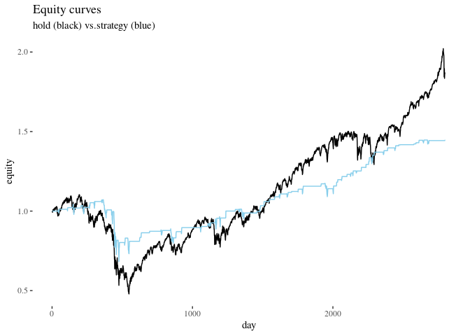
The result of your strategy is in blue. Note the flat lines: these are the times when your strategy stops you from being on the market. You avoid some drawdowns, but you also avoid making money on some strong positive trends. Crucially, the final equities for the two ways to proceed are:

tail(equityHold,1)

## [1] 1.869234

tail(equityStrategy,1)

## [1] 1.446046

But perhaps you’re not too worried, because you think that you can use your capital on some other markets for the idle days and so in the end your money would we working for you more than 15% of the time. Sure.

Center your returns!

So suppose what we care about is average daily returns and we’re not worried about how many days the strategy tells you to be on the market as long as its a fairly decent exposure time. Here is a problem. When you you looked at average returns, and these can be simply positive because the market went up over the years. The question is, whether your strategy would allow you to beat the market, and to evaluate this better you need to center the returns so that they average to zero and then look at what gain you’d expect from your strategy in terms of the centered returns, including using centered returns in statistical significance estmation (read on for details). So, by how much would you have beaten, expectedly, the market per year if you’re only using your resources for US500?

returnsC  <- US500withSignal$retC[US500withSignal$signal == 1]
(1+mean(returnsC))^31

## [1] 1.022951

#as compared to holding the whole year
(1+mean(US500withSignal$retC))^200

## [1] 1

This, still is a bit of cheating as we repeatedly used the mean return in the calcuations instead of using all the centered returns that were used in the exposure. So, again, let’s look at extra equity lines which represent how you would stand compared to the market.

equityHoldC <- numeric(nrow(US500withSignal))
equityHoldC[1] <- 1
for (i in 2: nrow(US500withSignal)) {equityHoldC[i] <-
                                    equityHoldC[i-1] * (1+ US500withSignal$retC[i])}


returnsFullC  <- ifelse(US500withSignal$signal == 1, US500withSignal$retC,0)
equityStrategyC <- numeric(nrow(US500withSignal))
equityStrategyC[1] <- 1
for (i in 2: nrow(US500withSignal)) {equityStrategyC[i] <-
  equityStrategyC[i-1] * (1+ returnsFullC[i])}

ggplot()+geom_line(aes(x = 1: nrow(US500withSignal), y = equityHoldC))+
  geom_line(aes(x = 1: nrow(US500withSignal), y = equityStrategyC), col = "skyblue")+
  theme_tufte()+xlab("day")+ylab("equity")+ggtitle("Extra equity curves", subtitle ="hold (black) vs.strategy (blue)")

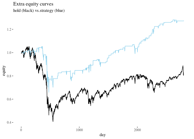
#compare mean daily returns:
mean(returnsC)

## [1] 0.0007322492

mean(US500withSignal$retC) #zero with rounding errors

## [1] 7.857887e-20

Ok. It doesn’t seem like you’re going to get rich soon, but at least this seems like progress, right? Right?

Comparison to random strategies

To get a clearer picture, let’s investigate whether the strategy does much better than just trading on random days, for the same number of days.

set.seed(123)
daily <- mean(returnsC)
n <- length(returnsC)

randomGains <- numeric(10000)
for(i in 1:10000){
randomDays <-   sample(US500withSignal$retC,n)
randomGains[i] <- mean(randomDays)
}


ggplot()+geom_histogram(aes(x=randomGains), bins = 50)+geom_vline(xintercept = daily)+theme_tufte()+
  labs(title = "Average daily gains for 10k random strategies", subtitle = "Average daily gain of your strategy marked with a vertical line")+xlab("daily gain")

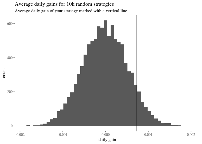
sum(randomGains >= daily)/length(randomGains)

## [1] 0.0799

This suggests that around 7% of random strategies would have done better than the carefully formulated one, and this casts some doubt on whether the latter is deeply superior. Here’s a more visual approach, where we plot extra equity curves including 20 random strategies:

 randomResults <- list()

 n <- length(returnsC)
 set.seed(123)
 for(i in 1:20){
 randomDays <- sample(2:nrow(US500withSignal),n)
 randomReturns <- numeric(nrow(US500withSignal))
 randomReturns[randomDays] <-  US500withSignal$retC[randomDays]

 randomEquity <- numeric(nrow(US500withSignal))
 randomEquity[1] <- 1
 for (d in 2: nrow(US500withSignal)) {
randomEquity[d] <- randomEquity[d-1] * (1+ randomReturns[d])
 }
 randomResults[[i]] <- randomEquity
 }

 ggplot()+geom_line(aes(x = 1: nrow(US500withSignal), y = equityHoldC))+
geom_line(aes(x = 1: nrow(US500withSignal), y = equityStrategyC), col = "skyblue")+
geom_line(aes(x = 1: nrow(US500withSignal), y = randomResults[[1]]), col = "gray")+
geom_line(aes(x = 1: nrow(US500withSignal), y = randomResults[[2]]), col = "gray")+
geom_line(aes(x = 1: nrow(US500withSignal), y = randomResults[[3]]), col = "gray")+
geom_line(aes(x = 1: nrow(US500withSignal), y = randomResults[[4]]), col = "gray")+
geom_line(aes(x = 1: nrow(US500withSignal), y = randomResults[[5]]), col = "gray")+
geom_line(aes(x = 1: nrow(US500withSignal), y = randomResults[[6]]), col = "gray")+
geom_line(aes(x = 1: nrow(US500withSignal), y = randomResults[[7]]), col = "gray")+
geom_line(aes(x = 1: nrow(US500withSignal), y = randomResults[[8]]), col = "gray")+
geom_line(aes(x = 1: nrow(US500withSignal), y = randomResults[[9]]), col = "gray")+
geom_line(aes(x = 1: nrow(US500withSignal), y = randomResults[[11]]), col = "gray")+
geom_line(aes(x = 1: nrow(US500withSignal), y = randomResults[[12]]), col = "gray")+
geom_line(aes(x = 1: nrow(US500withSignal), y = randomResults[[13]]), col = "gray")+
geom_line(aes(x = 1: nrow(US500withSignal), y = randomResults[[14]]), col = "gray")+
geom_line(aes(x = 1: nrow(US500withSignal), y = randomResults[[15]]), col = "gray")+
geom_line(aes(x = 1: nrow(US500withSignal), y = randomResults[[16]]), col = "gray")+
geom_line(aes(x = 1: nrow(US500withSignal), y = randomResults[[17]]), col = "gray")+
geom_line(aes(x = 1: nrow(US500withSignal), y = randomResults[[18]]), col = "gray")+
geom_line(aes(x = 1: nrow(US500withSignal), y = randomResults[[19]]), col = "gray")+
geom_line(aes(x = 1: nrow(US500withSignal), y = randomResults[[20]]), col = "gray")+
theme_tufte()+xlab("day")+ylab("equity")+ggtitle("Extra equity curves including 20 random strategies", subtitle ="hold (black) vs. strategy (blue) random (gray)")

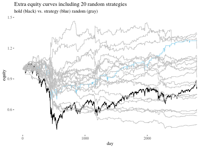
Conceptual point: the extra equity curve illustrates what would have happened with your equity if the only returns were those above the marked progress tracked by what happens to the buying and holding strategy. For this reason, the buying and holding extra equity ends up lower than 1. After all, the mean of centered returns is 0. To take a simple example, say you only have consider two days with centered returns $(-0.1,0.1)$. The mean is zero, but the extra equity is $1\times 0.9 \times 1.1 = 0.99$. If you lose $10\%$, you need to gain more than $10\%$ of what you now have to get back to your original equity.

Evaluation using the test set

Now, let’s run the same analysis on the test data.

US500test$ret <- numeric(nrow(US500test))
for(r in 1:nrow(US500test)){
  US500test$ret[r] <- (US500test$open[r+2]/US500test$open[r+1])-1
}
US500test$ret[(nrow(US500test)-1):nrow(US500test)] <- rep(0,2)
US500test$retC <- US500test$ret - mean(US500test$ret, na.rm=TRUE)

US500test <- signal(US500test)
returnsCtest  <- US500test$retC[US500test$signal == 1]

annualOnMarketTest <- round(length(returnsCtest)/nrow(US500test) *200)

#expected improvement annualized
(1+mean(returnsCtest))^annualOnMarketTest

## [1] 1.006072

#now comparison with random strategies
set.seed(123)
daily <- mean(returnsCtest)

n <- length(returnsCtest)

randomGainstest <- numeric(10000)
for(i in 1:10000){
  randomDaystest <-   sample(US500test$retC,n)
  randomGainstest[i] <- mean(randomDaystest)
}


ggplot()+geom_histogram(aes(x=randomGainstest), bins = 50)+geom_vline(xintercept = daily)+theme_tufte()+
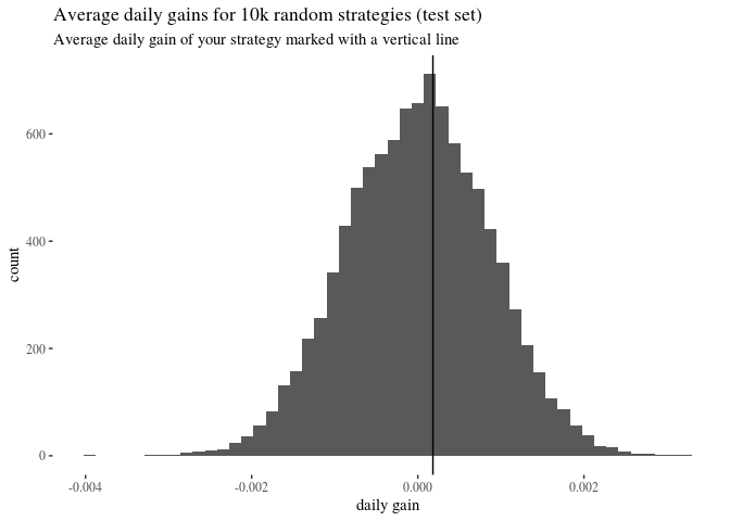
  labs(title = "Average daily gains for 10k random strategies (test set)", subtitle = "Average daily gain of your strategy marked with a vertical line")+xlab("daily gain")

#what's the relative frequency of random strategies that do better?
sum(randomGainstest >= daily)/length(randomGainstest)

## [1] 0.4184

We can also plot extra equities for our strategy, buying and holding, and a bunch of random equities.

randomResultstest <- list()

n <- length(returnsCtest)
set.seed(123)
for(i in 1:20){
randomDaystest <- sample(2:nrow(US500test),n)
randomReturnstest <- numeric(nrow(US500test))
randomReturnstest[randomDaystest] <-  US500test$retC[randomDaystest]

randomEquitytest <- numeric(nrow(US500test))
randomEquitytest[1] <- 1
for (d in 2: nrow(US500test)) {
  randomEquitytest[d] <- randomEquitytest[d-1] * (1+ randomReturnstest[d])
}
randomResultstest[[i]] <- randomEquitytest
}

equityHoldCtest <- numeric(nrow(US500test))
equityHoldCtest[1] <- 1
for (i in 2: nrow(US500test)) {equityHoldCtest[i] <-
                                    equityHoldCtest[i-1] * (1+ US500test$retC[i])}

returnsFullCtest  <- ifelse(US500test$signal == 1, US500test$retC,0)

equityStrategyCtest <- numeric(nrow(US500test))
equityStrategyCtest[1] <- 1
for (i in 2: nrow(US500test)) {equityStrategyCtest[i] <-
  equityStrategyCtest[i-1] * (1+ returnsFullCtest[i])}



ggplot()+geom_line(aes(x = 1: nrow(US500test), y = equityHoldCtest))+
  geom_line(aes(x = 1: nrow(US500test), y = equityStrategyCtest), col = "skyblue")+
  geom_line(aes(x = 1: nrow(US500test), y = randomResultstest[[1]]), col = "gray")+
  geom_line(aes(x = 1: nrow(US500test), y = randomResultstest[[2]]), col = "gray")+
  geom_line(aes(x = 1: nrow(US500test), y = randomResultstest[[3]]), col = "gray")+
  geom_line(aes(x = 1: nrow(US500test), y = randomResultstest[[4]]), col = "gray")+
  geom_line(aes(x = 1: nrow(US500test), y = randomResultstest[[5]]), col = "gray")+
  geom_line(aes(x = 1: nrow(US500test), y = randomResultstest[[6]]), col = "gray")+
  geom_line(aes(x = 1: nrow(US500test), y = randomResultstest[[7]]), col = "gray")+
  geom_line(aes(x = 1: nrow(US500test), y = randomResultstest[[8]]), col = "gray")+
  geom_line(aes(x = 1: nrow(US500test), y = randomResultstest[[9]]), col = "gray")+
  geom_line(aes(x = 1: nrow(US500test), y = randomResultstest[[11]]), col = "gray")+
  geom_line(aes(x = 1: nrow(US500test), y = randomResultstest[[12]]), col = "gray")+
  geom_line(aes(x = 1: nrow(US500test), y = randomResultstest[[13]]), col = "gray")+
  geom_line(aes(x = 1: nrow(US500test), y = randomResultstest[[14]]), col = "gray")+
  geom_line(aes(x = 1: nrow(US500test), y = randomResultstest[[15]]), col = "gray")+
  geom_line(aes(x = 1: nrow(US500test), y = randomResultstest[[16]]), col = "gray")+
  geom_line(aes(x = 1: nrow(US500test), y = randomResultstest[[17]]), col = "gray")+
  geom_line(aes(x = 1: nrow(US500test), y = randomResultstest[[18]]), col = "gray")+
  geom_line(aes(x = 1: nrow(US500test), y = randomResultstest[[19]]), col = "gray")+
  geom_line(aes(x = 1: nrow(US500test), y = randomResultstest[[20]]), col = "gray")+
  theme_tufte()+xlab("day")+ylab("equity")+ggtitle("Extra equity curves including 20 random strategies (test set)", subtitle ="hold (black) vs. strategy (blue) random (gray)")

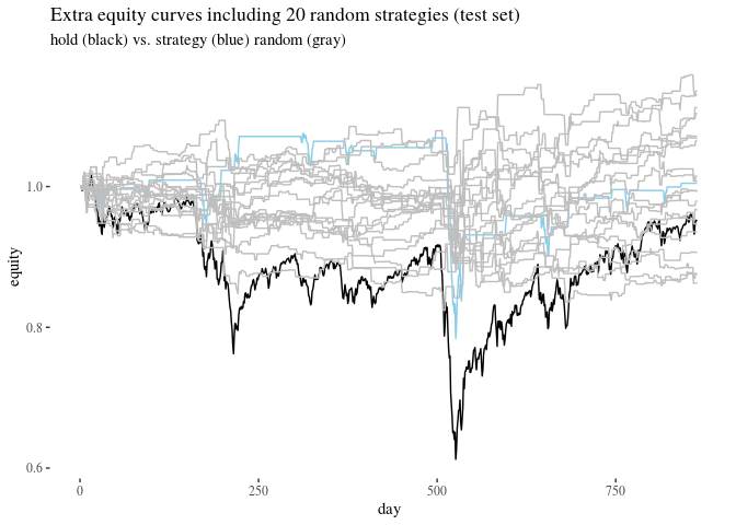
Are you still impressed?

Optimization

But hey, maybe the signaling parameters weren’t too good. Let’s try to optimize them.

#create table with candidates
lookbackOptions <- c(9,15,18,20,22,25)
multiplierOptions <- c(2.1,2,1.9,1.8,1.7,1.6,1.5)

options <- expand.grid(lookbackOptions,multiplierOptions)
colnames(options) <- c("lookbackOptions","multiplierOptions")

#note there are quite a few, so the computation might take a bit
nrow(options)

## [1] 42

#let's calculate avg daily gains for each of this signaling strategies
#this might take a while
options$dailyGains <- numeric(nrow(options))

for (option in 1: nrow(options)){

  US500new <- signal(US500, lookback = options$lookbackOptions[option],
                            multiplier = options$multiplierOptions[option])

  newGains <- US500new$retC[US500new$signal == 1]

  options$dailyGains[option] <- mean(newGains)
}

#and let's sort them to have the best ones on top
optionsSorted <- options[order(options$dailyGains, decreasing = TRUE),]

#inspect
head(optionsSorted)

##    lookbackOptions multiplierOptions   dailyGains
## 30              25               1.7 0.0010182723
## 25               9               1.7 0.0010109784
## 26              15               1.7 0.0009911704
## 12              25               2.0 0.0008912633
## 35              22               1.6 0.0008378764
## 18              25               1.9 0.0008199543

#how does the best option do?
topDaily <- optionsSorted[1,3]

topDaily/daily

## [1] 5.381827

Woah, that’s more than five times better than the old one, right? so you’re like, aha, let’s use lookback 25 and multiplier 1.7!

Testing the optimized strategy

What happens when you compare this to random strategies? You might be inlined to simply repeat the previous analysis:

#plug it in
US500optimal <- signal(US500, lookback = 25, multiplier = 1.7)
returnsCoptimal  <- US500optimal$retC[US500optimal$signal == 1]
GAIN <- mean(returnsCoptimal)
GAIN

## [1] 0.001018272

ggplot()+geom_histogram(aes(x=randomGains), bins = 50)+geom_vline(xintercept = GAIN)+theme_tufte()+
  labs(title = "Average daily gains for 10k random strategies", subtitle = "Average daily gain of the optimal strategy marked with a vertical line")+xlab("daily gain")

sum(randomGains >= GAIN)/length(randomGains)

## [1] 0.0245

Right on! Now your strategy is better than around $98\%$ random strategies, which seems pretty cool!

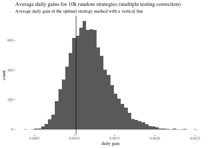
But wait. Note that this time you tested 42 different strategies and chose the best one, so you need to correct for multiple testing. Your bootstrapping evaluation should mimic this. So instead of comparison to a bunch of random stragies, you should every time get 42 random strategies and pick the best one as a potential candidate. Like this:

n <- length(returnsCoptimal)
randomGainsMax42 <- numeric(10000)
for(g in 1:10000){
    group <- numeric(42)
    for (s in 1:42){
      randomDays <-   sample(US500optimal$retC,n)
      group[s] <-     mean(randomDays)
      randomGainsMax42[g] <- max(group)
          }
}


ggplot()+geom_histogram(aes(x=randomGainsMax42), bins = 50)+geom_vline(xintercept = GAIN)+theme_tufte()+
  labs(title = "Average daily gains for 10k random strategies (multiple testing correction)", subtitle = "Average daily gain of the optimal strategy marked with a vertical line")+xlab("daily gain")

sum(randomGainsMax42 > GAIN)/length(randomGainsMax42)

## [1] 0.7338

This is slightly less impressive. If instead of coming up with a meticulous list of potential parameter combinations and optimizing, you simply randomly generated 42 random strategies, the best of those would around $73\%$ of the time do better than the one you obtained by optimizing. Huh.